Complex Disordered Systems

Arrested states: Glasses

Francesco Turci

Today

• Equilibrium and nonequilibrium
• Energy landscapes
• Glasses

Equilibrium

Equilibrium means:

• no change in entropy wirh time (zero entropy production)

• no net flows of matter or energy

• detailed balance \pi_i P_{i \rightarrow j} = \pi_j P_{j \rightarrow i}

• time reversibility

• state of maximum entropy given the constraints (we saw this in multiple instances, e.g. liquid crystals)

• macroscopic obserbvables do not change with time (stationarity)

• equivalence between time and ensemble averages (ergodicity)

Ergodicity

Let’s focus a moment on ergodicity.

• The basic idea is that we are performing a measurement. This takes time: the observation time t_{obs}.
• If the system is ergodic, then the time average over t_{obs} is equivalent to an ensemble average over many copies of the system at a fixed time.

\overline{A} = \frac{1}{t_{obs}} \int_{0}^{t_{obs}} A(t) dt = \langle A \rangle

• It is important that then t_{obs} needs to be large enough for the system to explore a large number of representative configurations:
  • the dynamics needs to sample the relevant parts of phase space in order to get an unbiased estimate of the average.
  • the dynamics has its own relaxation timescales \tau that need to be considered.
• Ergodicity is typically assumed, but it is a strong assumption.

Equilibration and relaxation

• Typically, a system requires time in order to reach equilibrium:
  • a system is prepared in some state at time t_0,
  • it is the put in contact with an environment that we assume to be thermal (fundamentally, a large system of which we know very little, for which we express our maximal ignorance by only tracking its temperature, pressure etc…)
  • then we let it evolve until it reaches equilibrium at time t_{eq}.
  • This equilibration time depends:
    • on the distance from equilibrium between the initial and final state
    • on the intrinsic dynamics of the system (its own relaxation time)

What could go wrong?

On the chalkboard, let’s list some issues that could arise during equilibration.

What could go wrong?

Phase space hard to explore
System gets stuck: the dynamics explores a local equilibrium region

Very slow evolution
The system keeps changing, it ages

Internal/external driving
Currents are generated and the system never equilibrates

Constrained dynamics
Some configurations are forbidden (constraints on the rules of motion) and non-ergodicity arises

Energy landscapes

• A system of many partcles has many degrees of freedom.
• The free energy is a scalar function of all these degrees of freedom: F(x_1, x_2, \ldots, x_N).
• We can think of it is the altitude of a landscape in a high-dimensional space.
• The landscape represents the (negative log) of the probability distribution of configurations: low energy = high probability.
  • it depends on the intensive parameters (temperature, pressure, etc..)

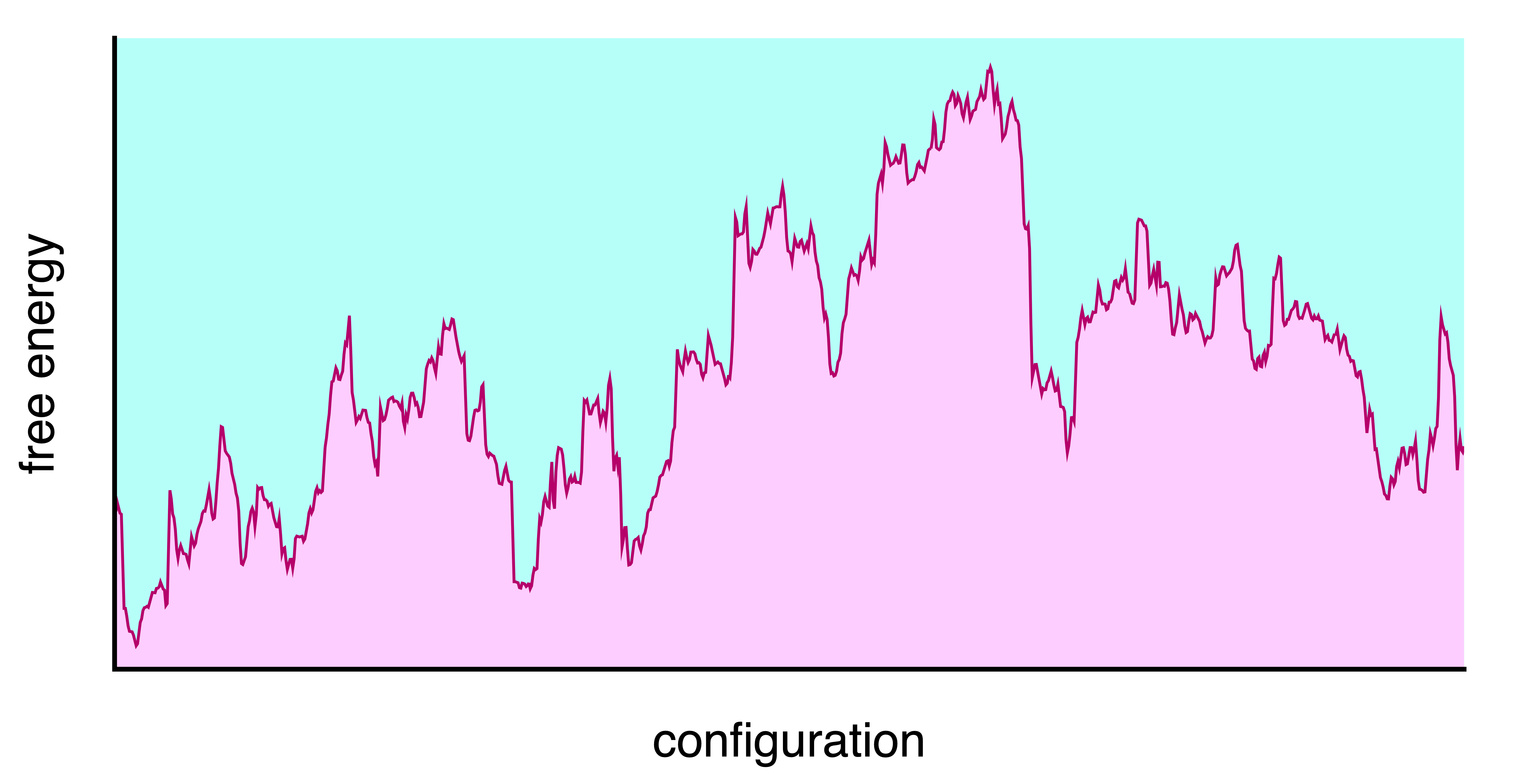
Free energy landscape of a complex system at some temperature T and pressure P

Energy landscapes

• Different minima correspond to different conformations or states of the system. (e.g. liquid/gas, crystal/amorphous solid, folded/unfolded protein)
• They are separated by energy barriers \Delta F
• The time to transition is often modelled as Arrhenius \tau \sim \exp\left(\dfrac{\Delta F}{k_{B} T}\right)

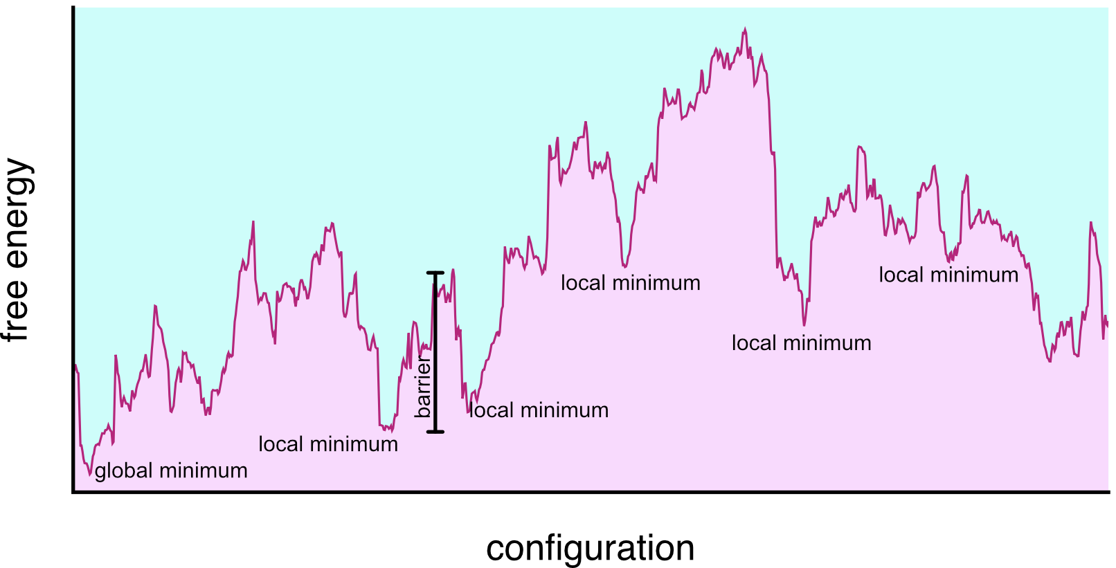
Minima in the free energy landscape

Metabasins

When the temperature allows it, connected minima can be grouped into single basins called metabasins.

• they are not just energy minima, they include entropy
• they can behave as bone-fide local equilibria
• These are akin to the metastable states.

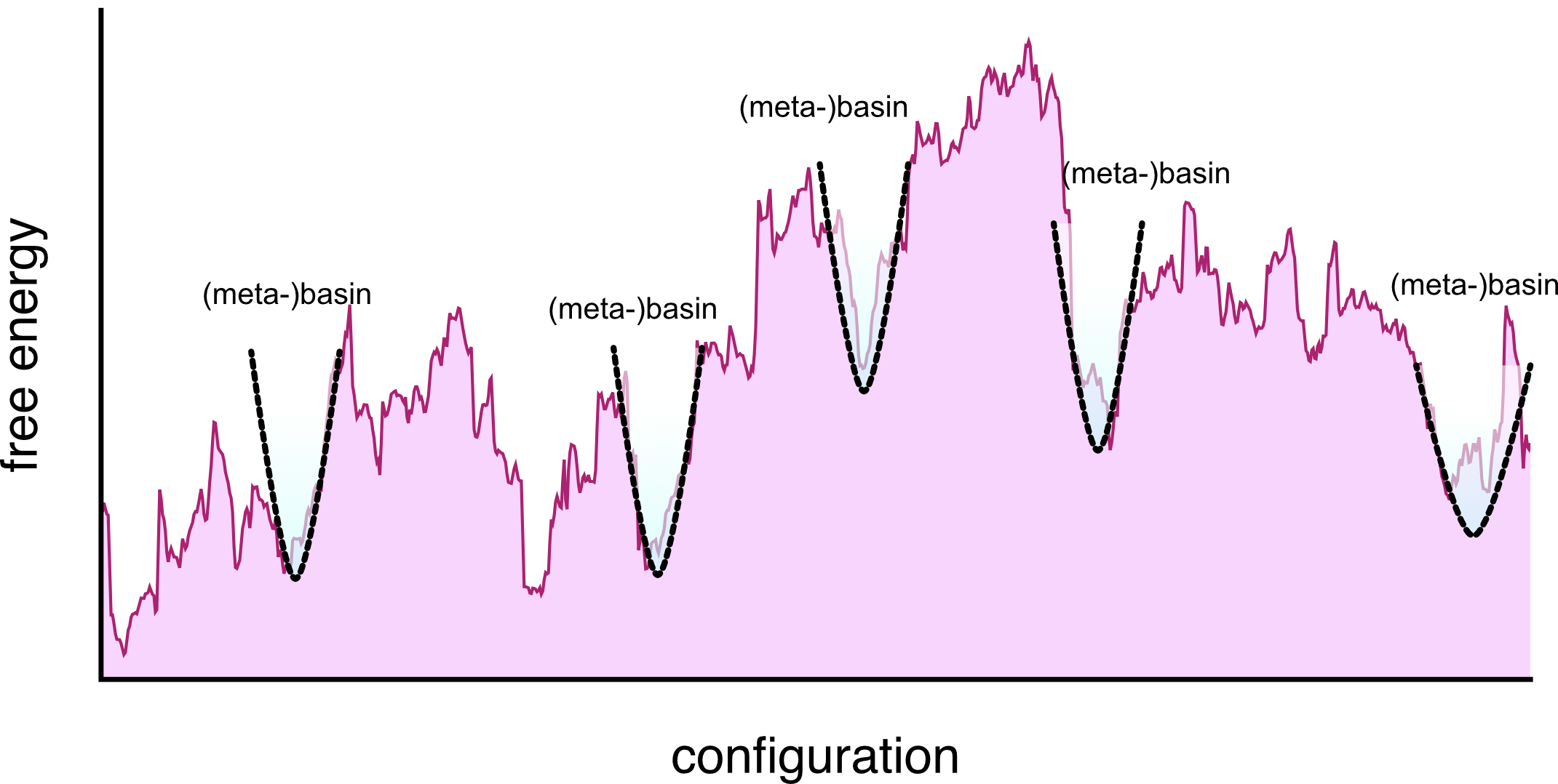
metabasins in the free energy landscape

Configurational entropy

• The number of distinct metabasins can be very large.
• We can define a configurational entropy S_{conf} that counts the number of distinct states \Omega: S_{conf} = k_{B} \ln N_{\mathrm minima}

Different from the total entropy S S(T) = S(T_0) + \int_{T_0}^{T} \frac{1}{T'} \left( \frac{\partial P}{\partial T'} \right)_V dV

or (at constant volume)

S(T) = S(T_0) + \int_{T_0}^{T} \frac{C_V(T')}{T'} dT' where C_V is the heat capacity at constant volume and T_0 is a reference temperature.

For gas, fluids, and liquids at high T only the total entropy is well defined.

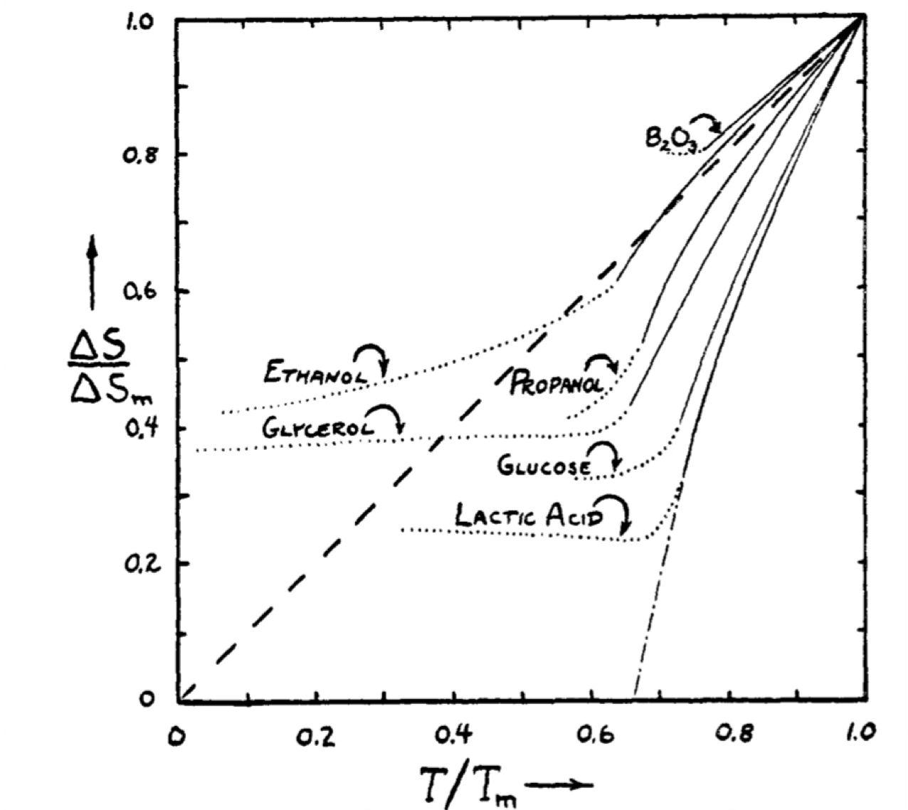
Configurational entropy

As we take liquids to low temperatures, we can separate the total entropy into a vibrational and configurational part and define S_{conf}(T) = S(T) -S_{vib}(T)

For several fluids, this decreases with temperature in an intriguing way.

[…] Perhaps in some instances a thermodynamic “freezing-in” of degrees of freedom does take place as a desperate result of the liquid’s excessive generosity with its limited supply of entropy and energy as its temperature is lowered below the melting point. This would imply the existence of some kind of state of high order for the liquid at low temperature which differs from the normal crystalline state. A plausible structure for such a state seems, however, difficult to conceive, and we believe that the paradox is better resolved in another way […] (W. Kauzmann, Chem. Rev. 43, 219 (1948)).

Kauzmann paradox: the entropy difference between the liquid and the crystal is extrapolated to low temperatures: glasses plateau, but what if we could equilibrate at very low T?

Glasses

Glassy systems are a broad class of systems, not necessarily atomic or molecular, that exhibit arrested dynamics

• upon changing a thermodynamic parameter (e.g. temperature, density) the system’s relaxation time \tau increases dramatically
• the system falls out of equilibrium and becomes non-ergodic
• the system behaves as a solid, but lacks long-range order (it is amorphous)

Glassformer	Scale of Constituents	Properties
Silicate glass	Atomic (Si, O atoms)	Strong, transparent, high melting point
Metallic glass	Atomic (metal atoms)	High strength, corrosion resistant, ductile
Polymer glass	Macromolecular (polymers)	Flexible, low density, tunable glass transition
Colloidal glass	Mesoscopic (colloids, ~nm–μm)	Opaque, tunable rheology, soft solid-like
Molecular glass	Molecular (organic molecules)	Low melting point, fragile, optical uses
Sugar glass	Molecular (sucrose, glucose)	Brittle, water soluble, low thermal stability
Chalcogenide glass	Atomic (S, Se, Te atoms)	Infrared transparency, phase-change memory

Glassy systems

But glassy physics is broader than glassy materials: dense assemblies in general will display glassy dynamics.

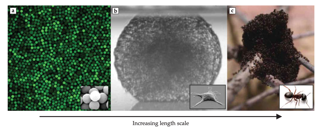
(a) Colloidal glasses, (b) dense cellular tissues, (c) ant colonies from Facets fo glassy physics, Berthier and Ediger, Physics Today (2016)

Glass formation

To form a glass we:

• start from the liquid at high temperature
• cool with a finite cooling rate fast enough to avoid crystallisation
• enter a local equilibrium state (the supercooled liquid)
• at some point the relaxation time \tau becomes longer than the experimental time scale and the system falls out of equilibrium into a glassy state
• changing the cooling rate changes the glass transition temperature T_g and the final glass properties

Glass formation tracked by specific volume, or enthalpy or configurational entropy (they all share the same behaviour)

Macroscopic Glass properties

• Glasses are solids: they have a finite shear modulus and yield stress
• Glasses are amorphous: they lack long-range order (no Bragg peaks in scattering experiments)
• Glasses are history-dependent: their properties depend on the cooling rate and thermal history
• Glasses exhibit ageing: their properties slowly evolve with time as they explore deeper minima in the energy landscape

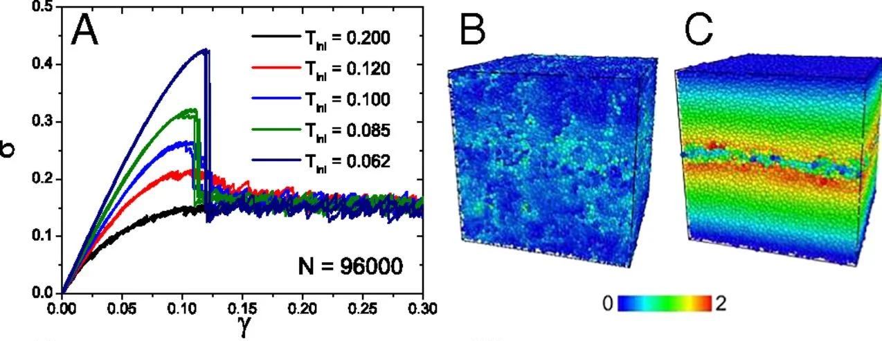
Example of brittle response in a simulated glassy model form Ozawa et al PNAS (2018): (a) stress-strain curves for different preparation temperatures; (b) initial deformation field, (b) final deformation field demonstrating fracture

Slowing down

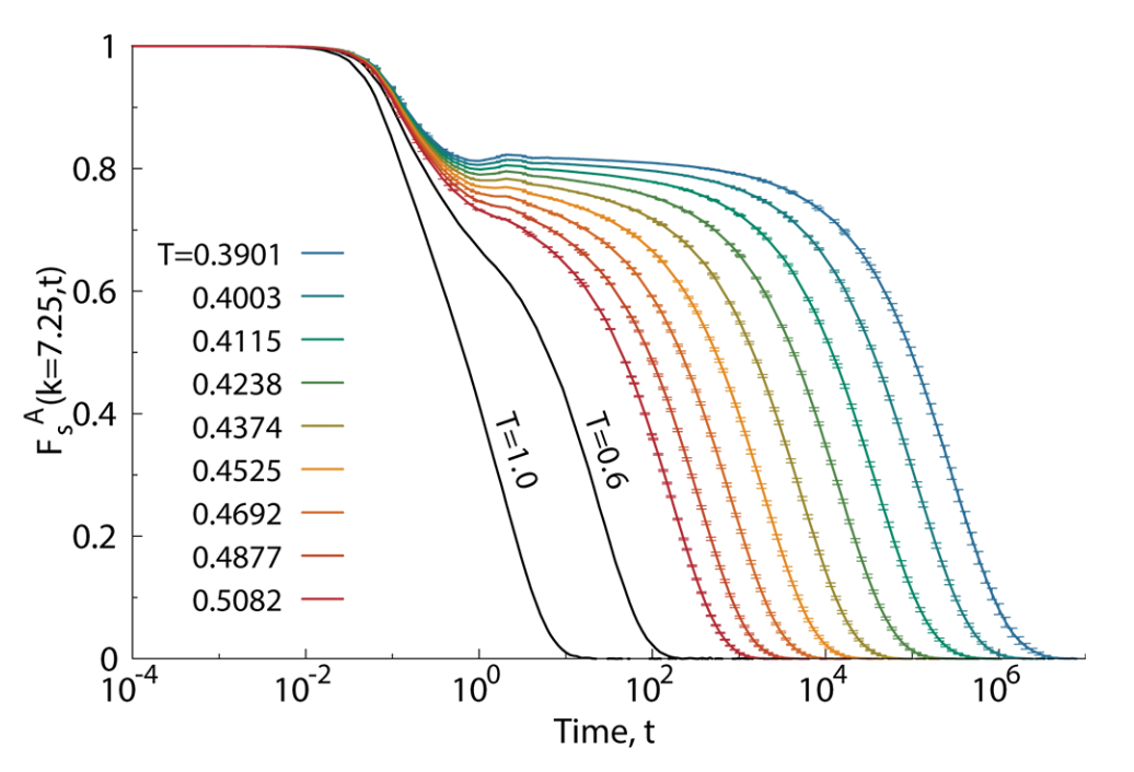
Their solid-like behavior arises from the dramatic slowing down of their dynamics as they approach the glass transition.

We quantify this with density autocorrelation functions such as the intermediate scattering function: F(k, t) = \frac{1}{N} \left\langle \sum_{j=1}^{N} e^{i \mathbf{k} \cdot [\mathbf{r}_j(t) - \mathbf{r}_j(0)]} \right\rangle

It decays in two steps:

• a fast decay corresponding to vibrations within the cage formed by neighbouring particles, occuring on a timescale called the beta relaxation time \tau_{\beta}
• a slow decay corresponding to structural relaxation as particles escape their cages, taking place on the much longer alpha relaxation time \tau_{\alpha}

Intermediate scattering function behaviour with lowering the temperature at a particular wave-vector corresponding to the first structural peak (first coordination shell), from Coslovich et al EPJE (2018)

Divergence of relaxation time and viscosity

The alpha relaxation time \tau_{\alpha} is proportional to the viscosity \eta and both increase dramatically as the temperature approaches the glass transition temperature T_g.

Phenomenologically one distinguishes between:

• Strong glassformers: Arrhenius behaviour of \tau_{\alpha} and \eta \sim \exp\left(\dfrac{E_a}{k_{B} T}\right)
• Fragile glassformers: super-Arrhenius behaviour \tau_{\alpha} and \eta. Often modelled with the Vogel-Fulcher-Tammann (VFT) equation \tau \sim \exp\left(\dfrac{A}{T - T_0}\right) where T_0 corrsponds to a divergence at finite temperature \to phase transition?

Angell plot showing the dramatic increase of viscosity and relaxation time as temperature approaches Tg for different glassformers, from Angell Science (1995)

Explaining the glass transition

• The glass transition is still not fully understood.
• It is one of the major open problems in condensed matter physics.

We have however various theories, mainly in two broad classes:

• Thermodynamic theories: posit an underlying phase transition at a temperature T_K (Kauzmann temperature) where the configurational entropy vanishes.
• Dynamic theories: attribute the slowing down to kinetic effects without invoking an underlying thermodynamic transition.

A thermodynamic theory: the Adam-Gibbs scenario

The Adam-Gibbs model links the dramatic slowdown of dynamics to the underlying thermodynamics through configurational entropy S_{\rm conf}.

• The key idea is the existense of cooperatively rearranging regions (CRRs): to relax, particles need to move together and explore a new metabasin in the energy landscape.

Mosaic of M_{CRR} independent cooperatively rearranging regions of size n_{CRR} particles each. The total number of particles is N = M_{CRR} n_{CRR}.

We assume that the total configurational entropy is additive and that each CRR contributes a constant amount s_{conf}, irrespective of its size

S_{conf} = M_{CRR} s^* = \dfrac{N}{n_{CRR}} s^*

Rearranging gives the size of a CRR as a function of the configurational entropy per particle S_{conf}/N: n_{CRR}(T) \propto \dfrac{1}{S_{conf}(T)/N}

Mosaic of cooperatively rearranging regions

A thermodynamic theory: the Adam-Gibbs scenario

We can then assume that the dynamics is activated with an energy barrier proportional to the size of a CRR:

\Delta E(T) \propto n_{CRR}(T)

From Arrhenius activation, the relaxation time is then

\tau_\alpha(T) = \tau_0 \exp\left(\frac{A}{T S_{\rm conf}(T)}\right)

As temperature decreases, S_{\rm conf} drops, causing \tau_\alpha to increase rapidly. If S_{\rm conf} vanishes at the Kauzmann temperature T_K, relaxation time diverges, reproducing the VFT form: \tau_\alpha(T) \sim \exp\left(\frac{B}{T - T_0}\right) with T_0 \approx T_K. This connects the kinetic slowdown to loss of configurational entropy making the theory thermodynamic.

It also points to a critical divergence: the size of the CRR needs to diverge as we approach T_K to have S_{conf} \to 0.

• Evidence for decreasing configurational entropy, but debated existence of a true thermodynamic transition.

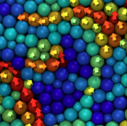
A dynamic theory: dynamical facilitation

Alternative model: glassy systems are universally heterogeneous in space and time: their mobility is very broadly distributed, with regions of high mobility coexisting with regions of low mobility.

This dynamical coexistence is called dynamical heterogeneity and can be formalised as a dynamical phase transition.

Key idea: Mobility facilitates more mobility

• Relaxation occurs only near already-mobile regions
• No underlying thermodynamic transition required

Temperature dependence:

• High T: Many mobile regions → fast relaxation
• Low T: Few mobile regions → cooperative motion required → slow relaxation

The relaxation time follows a parabolic law \log \tau_\alpha(T) \sim J^2 \left( \frac{1}{T} - \frac{1}{T_0} \right)^2

Unlike VFT, no finite-temperature divergence, no criticality, but still captures super-Arrhenius behavior.

- Recent evidence suggests facilitation as a dominating mechanism for relaxation at low temperatures.

Demonstration of facilitated dynamics and dynamical heterogeneities

Time evolution of the magnitude of the displacement field in a model of glass governed by dynamical facilitation from Hasym and Mandadapu PNAS (2024):

Excitations emerge and trigger further mobility in their vicinity, leading to a cascade of relaxation events.

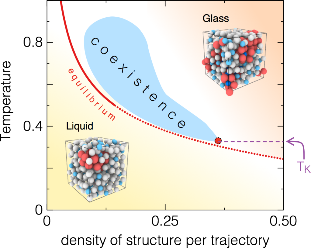
Unification

• Much more to glassy dynamics:
  • geometrical frustration
  • local structures
  • growth of lengthscales
  • jamming
  • mean field solutions (see Nobel Prize Giorgio Parisi)

Ongoing work to unify the various scenarios.

• Example: Turci et al PRX (2017): a numerical demonstration that an extension dynamical facilitation is compatible with decreasing entropies, emergence of local structures and criticality.

Phase diagram for structural-dynamical coexistence in glasses.