Geometries in active wetting

Tuneable repulsive barriers acting on phase-separated active Brownian particles lead to transitions analogous to complete to partial wetting in equilibrium.

The original geometry of the 2021 PRL consisted of a single barrier in an elongated box that promoted phase separation.

Here we explore different geometries, with the aim to stabilise droplet-like structures (if possible).

Geometry 1: the cross

The simplest modification we consider is to couple two barriers in the x and y direction of the simulation box. For convenience, $\varepsilon$ identifies the barrier strength. The simulations are run for a total of $200\tau_r$ rotational diffusion times, which is enough to attain a steady state in most conditions (but we may want to run even longer simulations to check the possibility of slow relaxation of the interfaces).

In two dimensions

In two dimensions, I observe the gradual transformation from a completely wet cross to the formation of accumulation in the corners of the cross, with large fluctuations from time frame to time frame and from quadrant to quadrant.

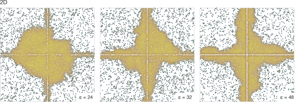
The fluctuations for weak barrier strengths are very strong, but it is maybe still possible to define time windows over which the density profiles in a quadrant are quasi-stationary

In three dimensions

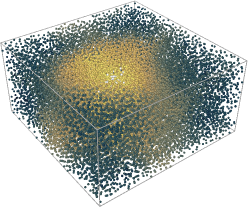
In this exploratory work - to save computation time - I have taken a system of unequal sizes $L_x = L_y= 2L_z = 40$. The dimension $z$ corresponds to the depth in the following plots and is therefore thinner than the other dimensions. This also make averages across z more significative as the geometry still promotes the slab instead of a sphere MIPS aggregate, as illustrated here below (the colour coding represents the local density within a cutoff radius at the second minimum of g(r), $3.1\sigma$).

We can look at lateral profiles to map the qualitative changes as the repulsive strength varies.

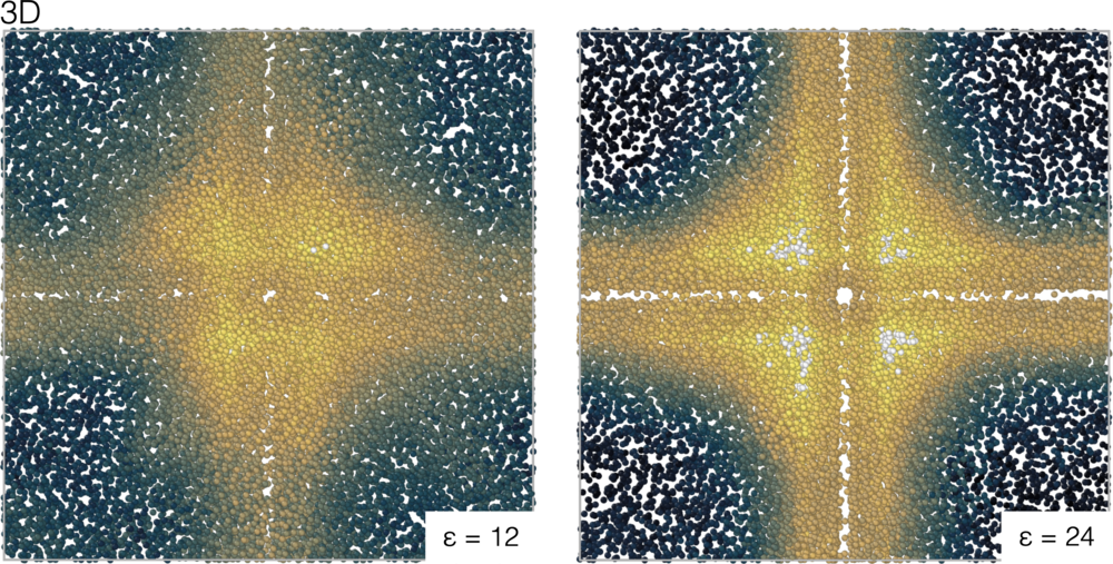
As $\varepsilon$ decreases, the profiles become more asymmetric and the density accumulates around the crossing point.

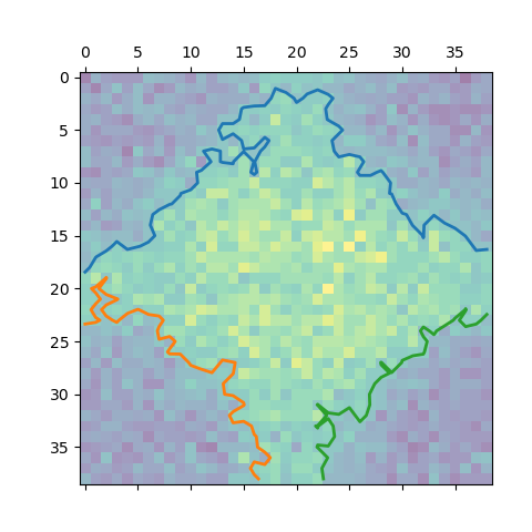
Even smaller $\varepsilon$ lead to the formation of a (strongly fluctuating) droplet that gets localised around the cross. For example, for $\varepsilon=8$ we have:

We can also identify a meaningful density contour. By choosing a suitable threshold (here $\rho=0.80$ ), we can separate the high and low-density regions and identify the (2d) projection of their lateral density profile

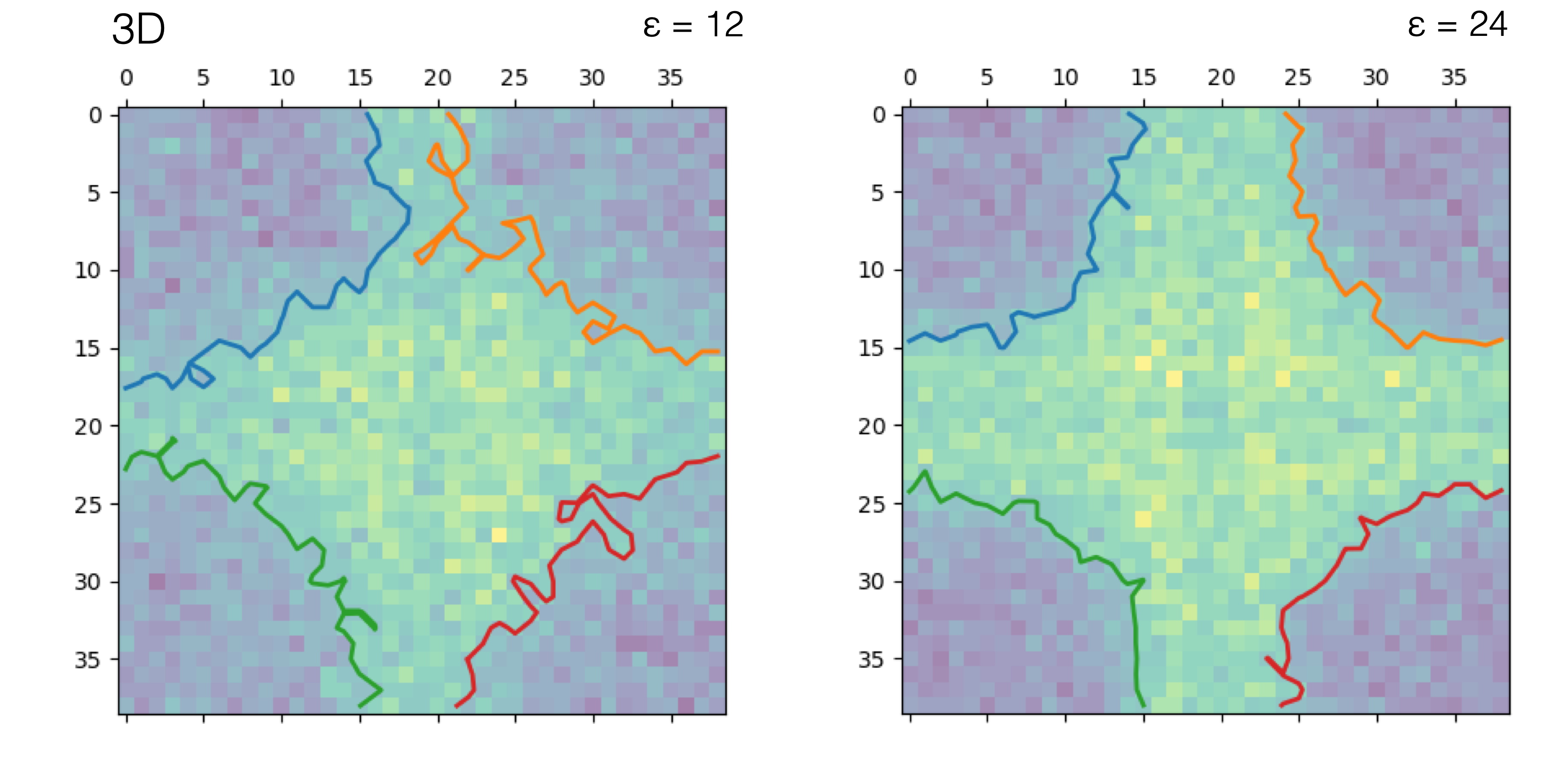
the contours fluctuate. They can - for example - cross the barrier.

Contour length

A simple quantity to describe the contours is the total length $\ell_{contour}$ which is the sum of all contours of each contour length. The quantity fluctuates significantly over the simulation, so here the bars represent standard deviations over the trajectory. Note that the (sharp) transition in 3d is around $\varepsilon\approx18-20$. Here we observe a gradual increase in the contour length that peaks around $\varepsilon=12$ and decreases below this value.

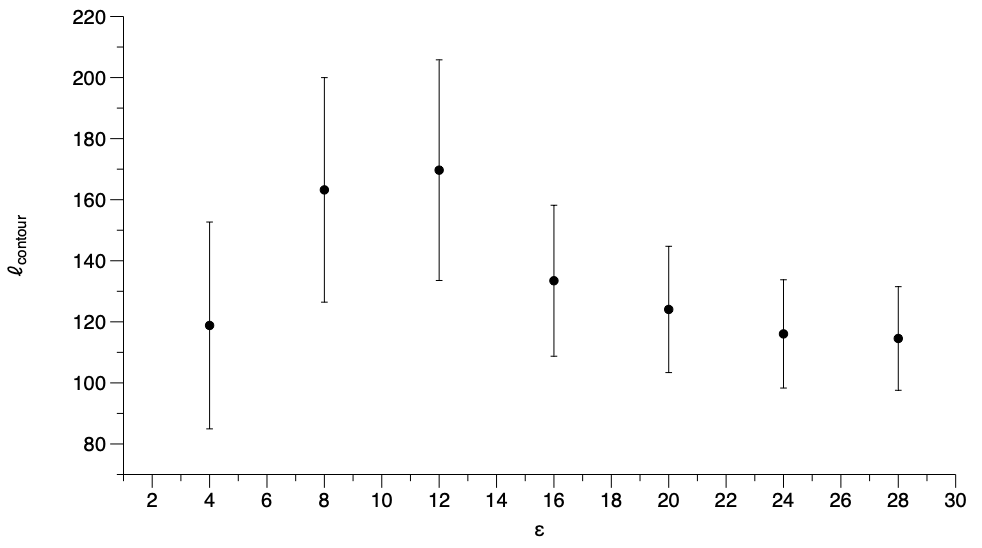
The decrease is due to a qualitative change: below $\varepsilon=12$ we mostly identify a single contour that never spans the system size. This suggests that some fine-tuning of the contour threshold may be required.

Asymmetry and finite size effects

A simple measure of asymmetry in the density distribution is the difference between the maximum and the minimum number of particles in a given quadrant of the cross. In terms of fractions of particles we have

\[\Delta_{\rm asym} (t)= \max_{i = 1...4} \{f_i\}(t)-\min_{i = 1...4}\{f_i\}(t)\]

where $i=1…4$ are the four quadrants of the cross. This difference can be averaged over time and compared for different system sizes.

Time series of the individual fractions are naturally noisy, for example in 3D

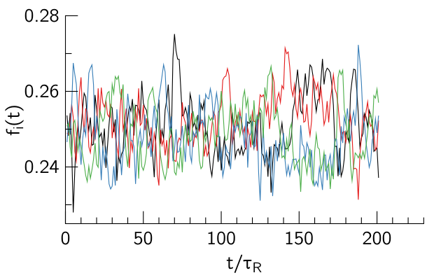
so I took averages after a (somewhat arbitrary) warmup time of 100 $\tau_R$.

For 2D systems, the simple metric of asymmetry seems to mix multiple effects:

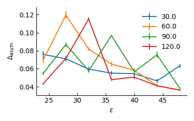
Chiefly, a possible issue may be due to trajectories that are too short: attaining the steady state becomes slower with decreasing $\varepsilon$ . Much longer averages (600 $\tau_R$) do not seem to address the issue

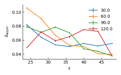
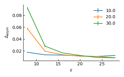
In the 3D case, it seems that the trends are clearer, with asymmetries that become larger at small $\varepsilon$ and smaller at large $\varepsilon$, which is reminiscent of the sharpening of the transition that I reported in the PRL,

Snapshots from larger systems

The larger systems also allow me to visualise the progressive change of the accumulated density around the crossing point.

For example, in 2D and 3D the asymmetry seems to be attained in pairs of quadrants (meaning that they are all coupled?)

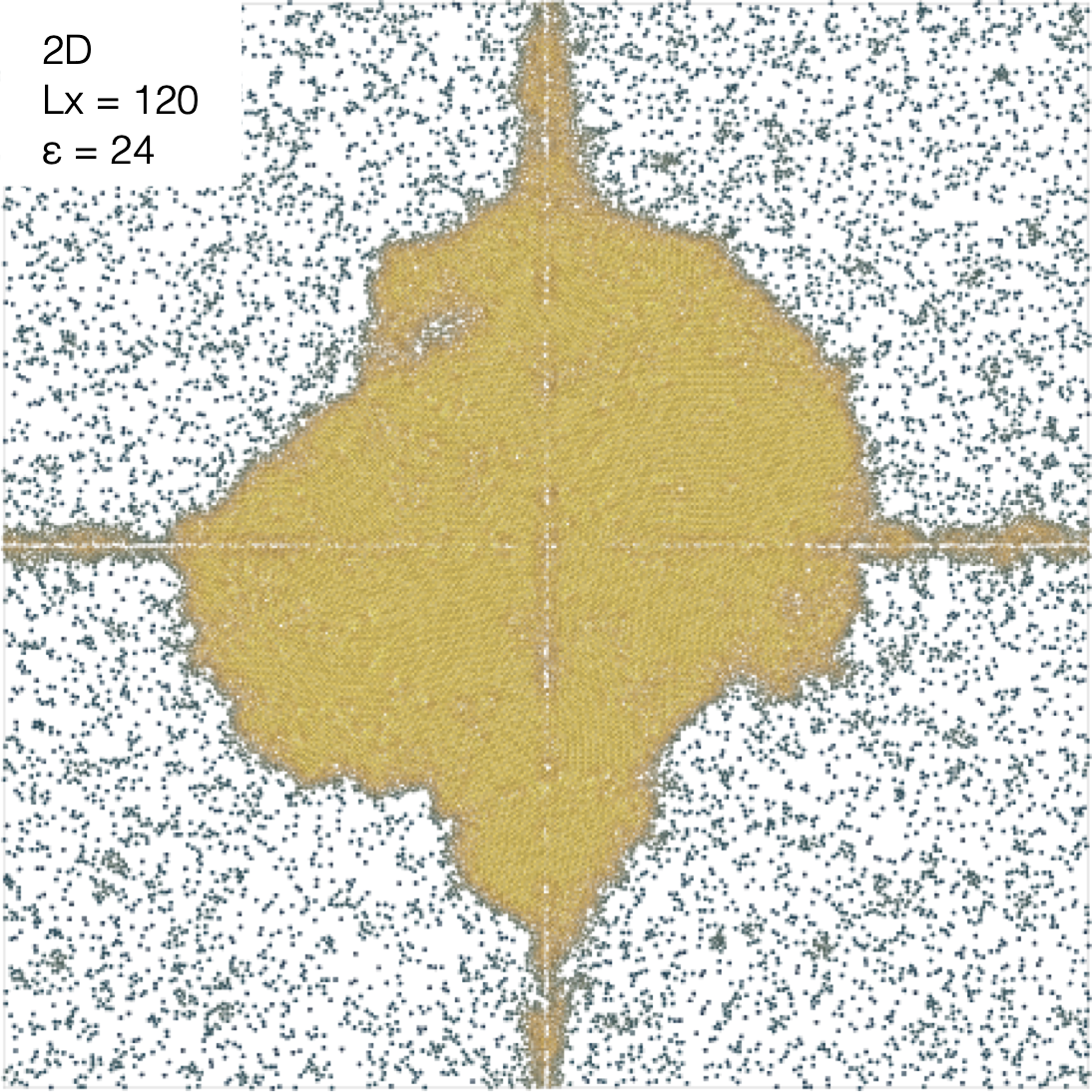
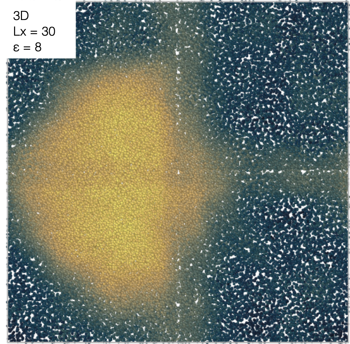
Note also that in both cases, the droplet-like sections seem to form an angle close to 90 degrees with the barriers (or it is an optical illusion).