Active wetting in corner geometry

Corner geometry

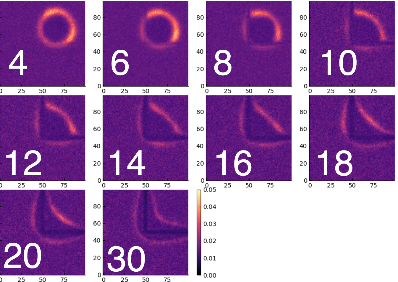
Running large simulations with $L_x=100\sigma$ for 700 $\tau_r$

$\varepsilon$	time average of the density
10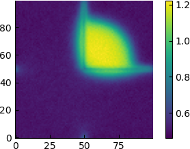
12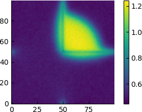
14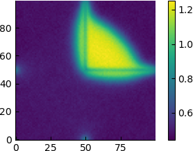
16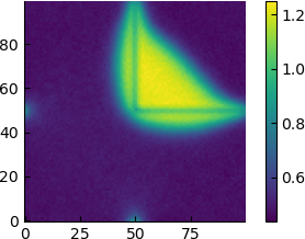
18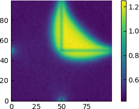
20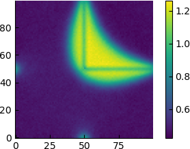
30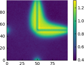

Note: there are significant finite size effects in the time required to nucleate the high density phase at small $\varepsilon$. For example. For example, for $\varepsilon=10$, I can observe the formation of MIPS and the “wetting” above but not for $L_x=40\sigma$, even after 1500 $\tau_r$, indicating that we are entering a regime dominated by homogeneous nucleation.

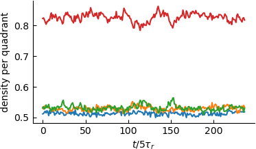
In fact, keeping $L_x=50\sigma$, we can decrease $\varepsilon$ further and see again that the time to observe MIPS becomes much longer. So, I can follow another route: I prepare a system at $\varepsilon=10$ and reduce the strength of the barrier instantaneously. What I observe is that the density is readjusted very rapidly, and the density per quadrant becomes stationary very quickly, e.g.

The pictures above would indicate that reducing the strength disfavours wetting and that around $\varepsilon=10$ we are in an almost neutral condition (the apparent contact angle is around 90 degrees). Can we get larger angles? Instantaneous snapshots of the system are intriguing, as in the following case at $\varepsilon=4$

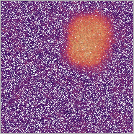
They would suggest thatthe droplet deforms and still its boundary would be modified by the presence of the wall, promoting contact in a region close to the corner and not away from it.

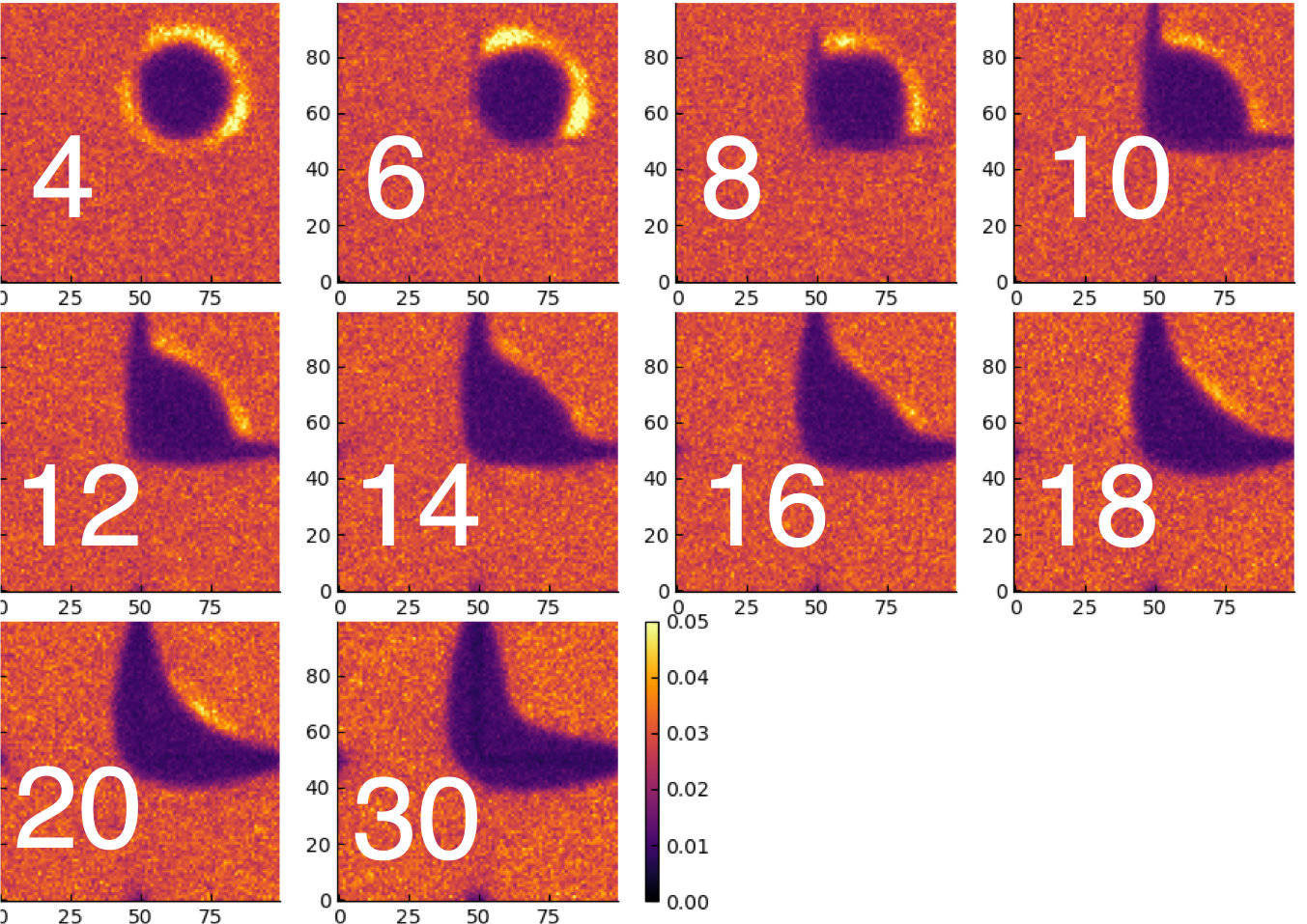
However, if we take a time-averaged picture we see the following

$\varepsilon$	Density
10
8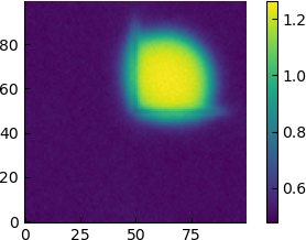
6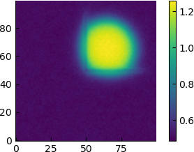
4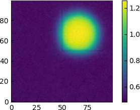

Seen from this point of view, it appears that the high-density region simply gradually distances itself from the barrier, and for $\varepsilon=6$ the average density profile already has a circular shape.

Further insight can be gleaned by looking at the density fluctuations. If we measure, for example, the variance of the density profiles, we observe a moderate increase in the variance as the strength is reduced

A pseud- compressibility can be obtained by rescaling the variance by the density,

The fluctuations are localised at the border, and most pronounced at the interface that is not in contact with the barrier.

Size of the fluctuations

To quantify the size of the fluctuation, I resort to a strategy similar to what I had done in the single barrier case: by trying to identify connected regions of relatively lower density within the high density phase.

I do so by :

• removing high-density regions (cutoff rcut = 2, coordination threshold = 40, meaning a local density of about 1.193~$\rho_{HD}$)
• clustering the remaining low density (short cutoff at 1.2 to separate the background from clusters inside the HD region)
• remove the largest cluster (most of the LD region) and uninteresting small clusters (either because they are too small or in the wrong quadrant).

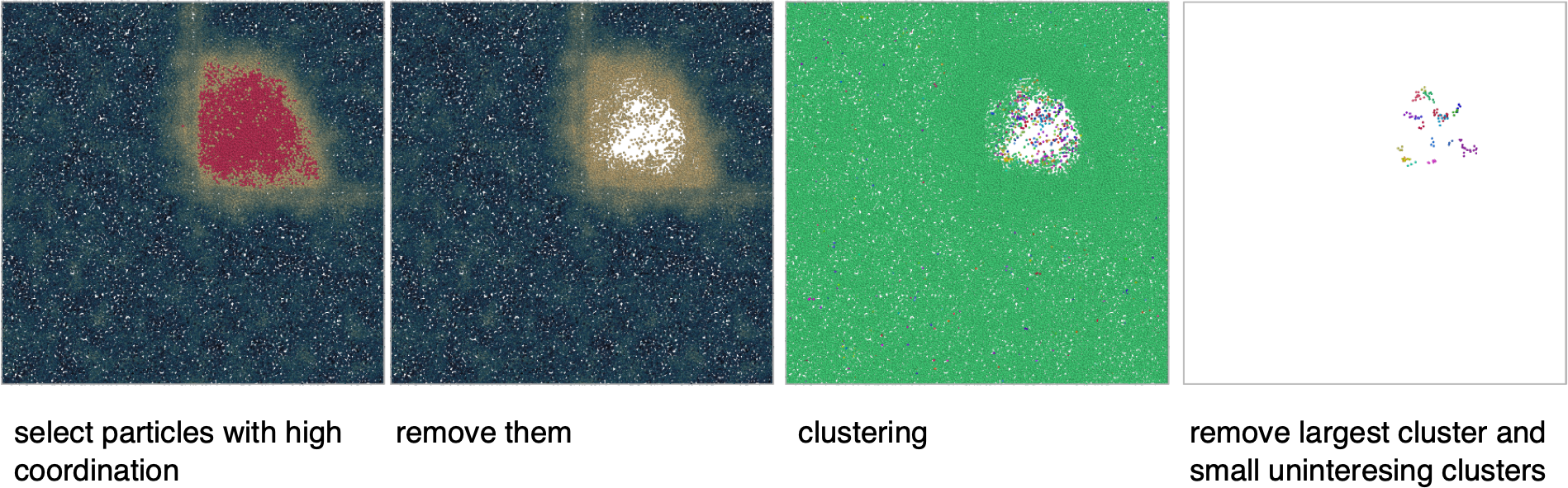
The resulting clusters of particles represent regions of low density within the high-density corner. Their size can be estimated using their radius of gyration.

The stationary probability distributions of the radius are characterised by exponential tails so that we can extract a meaningful average size. Here below, we see that this size increases progressively as the barrier strength is reduced.

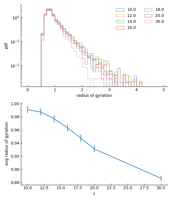
So this length scale increases very modestly (~12%) but it does increase. I can compare these increases to integral measures of the fluctuations plots above. So, I integrate (sum) the variance and the pseudo-compressibility $\chi=\rm{Var[\rho]}/\rm{Avg[\rho]}$ and plot their $\varepsilon$ dependence.

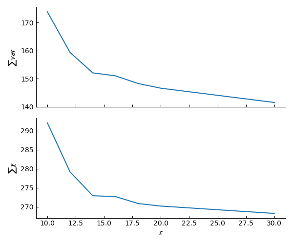
Here the changes seem to be sharper and more localised around $\varepsilon=10$. Yet, the ratios between extremes are similar: the integrated variance increases by 20% while the integrated $\chi$ increase by about 10% from high to low $\varepsilon$.

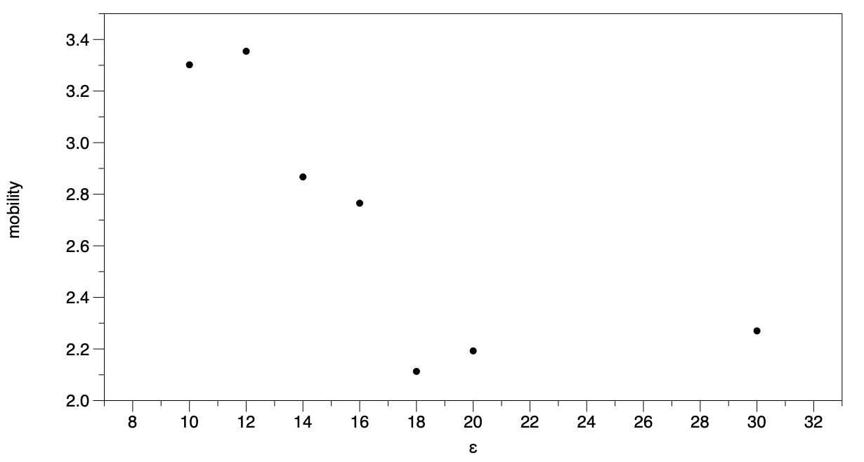
Mobility

Another possible source of fluctuations could be the enhanced mobility of the droplet. If we track the mean squared displacement of the centre of mass, we see that this remains localised

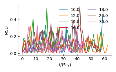
A better measure is the mobility of the centre of mass, defined as

\[k(\varepsilon) =\frac{1}{T-1}\sum_{t=1}^{T-1} |\mathbf{r}_{com}(t)-\mathbf{r}_{com}(t-1)|^2\]

The numerical evidence (albeit noisy) points towards an increase with decreasing $\varepsilon$