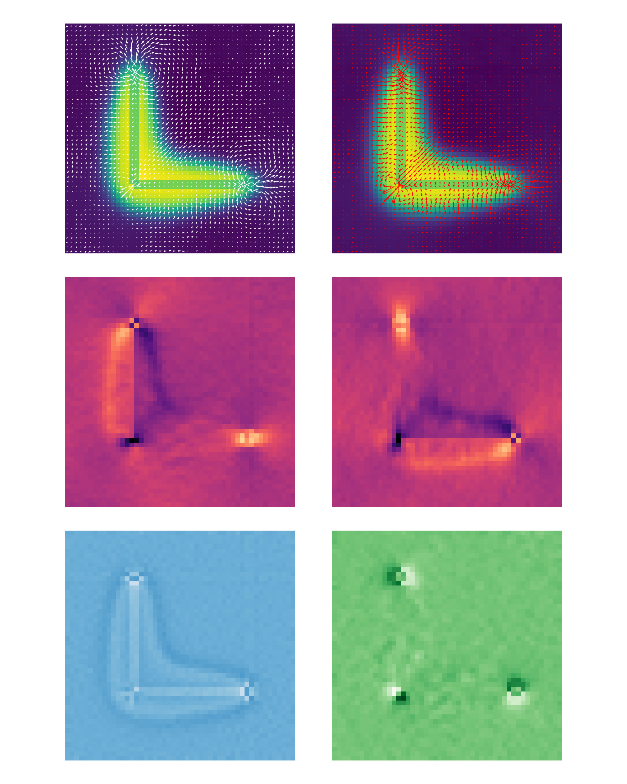
Fluxes in ABPs around a corner
Here I illustrate some numerical results on particle currents in the active system around the corner geometry.
To do so, I measure the displacements and take binned statistics of their components and of the number of particles, so that, for every sub volume $i$ of a suitable mesh.
So
$n_i =\sum_{j=1}^N \Lambda_i(\vec{r}_j )$
where $\Lambda_i(\vec{r}_j)$ is an indicator function which 0 or 1 depending on whether $\vec{r}_j$ is inside subvolume $i$ or not, and the components of the flux are (for example, the x component)
\[(F_x)_i =\sum_{j=1}^N \Lambda_i(\vec{r}_j) (\Delta\vec{r}_j)_x\]where $\Delta \vec{r}_j$ is the displacement. The average velocities per sub volume is then
$(v_x)_i=(F_x)_i/n_i\Delta t$
I then perform steady state averaging as well as averaging across the z direction (the thickness of these quasi-2d systems). I then compute the vector fields in the x, y plane overplayed with an average density profile, as well as the(z-averaged) $F_x,F_y$ components of the flow field and their divergence and curl.
Strong barrier $\varepsilon=30$
Intermediate barrier $\varepsilon=20$

Weak barrier $\varepsilon=10$
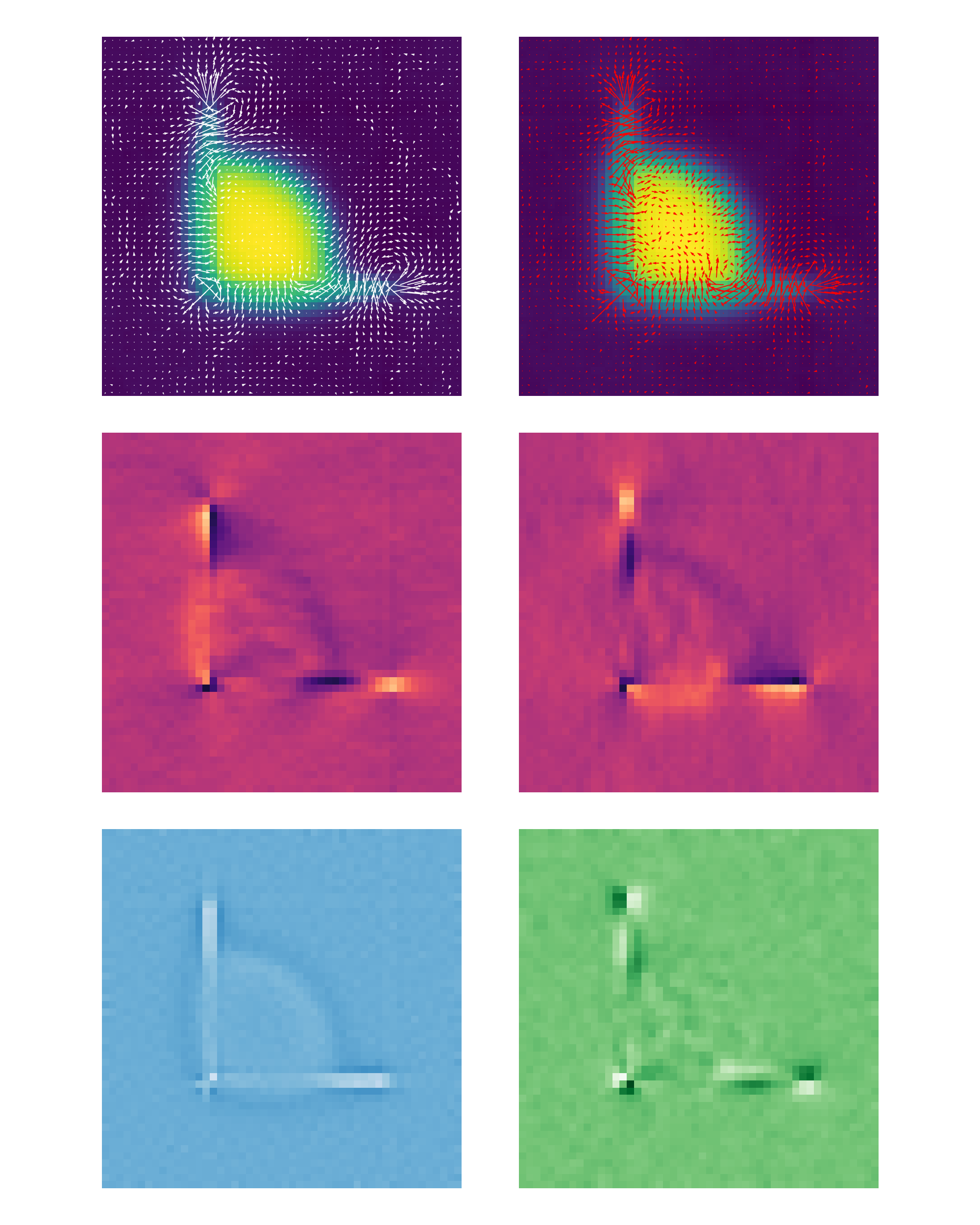
Remarks:
- There are nontrivial fluxes: particles are advected from the low density to the high density away from the obstacle and flow around the obstacle in its vicinity.
- The curl (and to some extent the e divergence) peak around the contact points
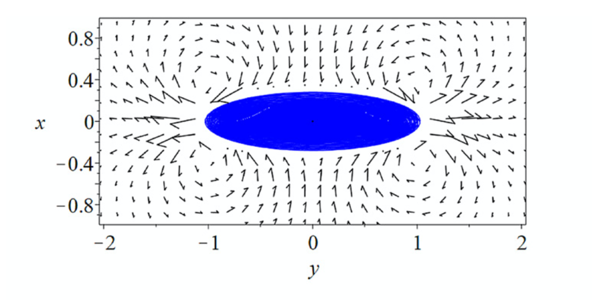
- The flow patterns for the more repulsive barries ($\varepsilon=30$) shares some similarities with the quadrupole around ellipsoidal obstacles (from Wagner et al. (2022). doi:10.1088/1742-5468/ac42cf ):