Example in jupyter

from __future__ import division
import numpy as np
from numpy.random import rand
import matplotlib.pyplot as plt


#----------------------------------------------------------------------
##  BLOCK OF FUNCTIONS USED IN THE MAIN CODE
#----------------------------------------------------------------------
def initialstate(N):   
    ''' generates a random spin configuration for initial condition'''
    state = 2*np.random.randint(2, size=(N,N))-1
    return state


def mcmove(config, beta):
    '''Monte Carlo move using Metropolis algorithm '''
    for i in range(N):
        for j in range(N):
                a = np.random.randint(0, N)
                b = np.random.randint(0, N)
                s =  config[a, b]
                nb = config[(a+1)%N,b] + config[a,(b+1)%N] + config[(a-1)%N,b] + config[a,(b-1)%N]
                cost = 2*s*nb
                if cost < 0:
                    s *= -1
                elif rand() < np.exp(-cost*beta):
                    s *= -1
                config[a, b] = s
    return config


def calcEnergy(config):
    '''Energy of a given configuration'''
    energy = 0
    for i in range(len(config)):
        for j in range(len(config)):
            S = config[i,j]
            nb = config[(i+1)%N, j] + config[i,(j+1)%N] + config[(i-1)%N, j] + config[i,(j-1)%N]
            energy += -nb*S
    return energy/4.


def calcMag(config):
    '''Magnetization of a given configuration'''
    mag = np.sum(config)
    return mag

## change these parameters for a smaller (faster) simulation 
nt      = 4         #  number of temperature points
N       = 8         #  size of the lattice, N x N
eqSteps = 1024       #  number of MC sweeps for equilibration
mcSteps = 1024       #  number of MC sweeps for calculation

T       = np.linspace(1.53, 3.28, nt) 
E,M,C,X = np.zeros(nt), np.zeros(nt), np.zeros(nt), np.zeros(nt)
n1, n2  = 1.0/(mcSteps*N*N), 1.0/(mcSteps*mcSteps*N*N) 
# divide by number of samples, and by system size to get intensive values

#----------------------------------------------------------------------
#  MAIN PART OF THE CODE
#----------------------------------------------------------------------
for tt in range(nt):
    print(tt)
    E1 = M1 = E2 = M2 = 0
    config = initialstate(N)
    iT=1.0/T[tt]; iT2=iT*iT;
    
    for i in range(eqSteps):         # equilibrate
        mcmove(config, iT)           # Monte Carlo moves

    for i in range(mcSteps):
        mcmove(config, iT)           
        Ene = calcEnergy(config)     # calculate the energy
        Mag = calcMag(config)        # calculate the magnetisation

        E1 = E1 + Ene
        M1 = M1 + Mag
        M2 = M2 + Mag*Mag 
        E2 = E2 + Ene*Ene

    E[tt] = n1*E1
    M[tt] = n1*M1
    C[tt] = (n1*E2 - n2*E1*E1)*iT2
    X[tt] = (n1*M2 - n2*M1*M1)*iT

0
1
2
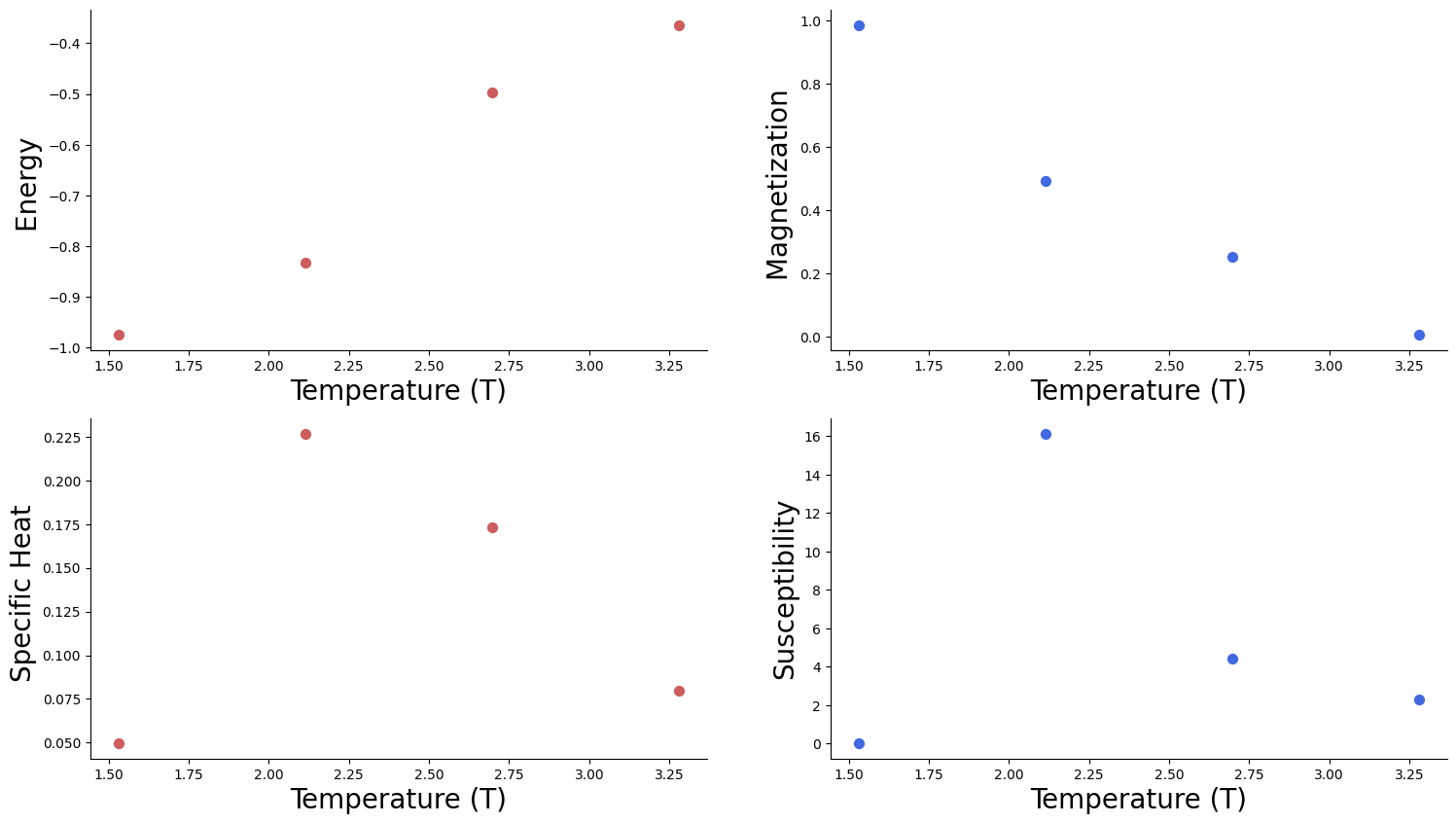
3

f = plt.figure(figsize=(18, 10)); # plot the calculated values    

sp =  f.add_subplot(2, 2, 1 );
plt.scatter(T, E, s=50, marker='o', color='IndianRed')
plt.xlabel("Temperature (T)", fontsize=20);
plt.ylabel("Energy ", fontsize=20);         plt.axis('tight');

sp =  f.add_subplot(2, 2, 2 );
plt.scatter(T, abs(M), s=50, marker='o', color='RoyalBlue')
plt.xlabel("Temperature (T)", fontsize=20); 
plt.ylabel("Magnetization ", fontsize=20);   plt.axis('tight');

sp =  f.add_subplot(2, 2, 3 );
plt.scatter(T, C, s=50, marker='o', color='IndianRed')
plt.xlabel("Temperature (T)", fontsize=20);  
plt.ylabel("Specific Heat ", fontsize=20);   plt.axis('tight');   

sp =  f.add_subplot(2, 2, 4 );
plt.scatter(T, X, s=50, marker='o', color='RoyalBlue')
plt.xlabel("Temperature (T)", fontsize=20); 
plt.ylabel("Susceptibility", fontsize=20);   plt.axis('tight');