Implementation of Vicsek dynamics

Aims

Initialise the start configuration with random positions and orientations
Specify the update rule specific to the Vicsek model

Learning outcomes

Using C++ random number generators
Updating objects’ properties

Random initial state

We have constructed all the objects we neeed:

a box
a set of particles
and a Simulation object to combined them together

We want now to think of our problem more concretely. First, our simulation needs to start from an initila configuration. This means that the particles composing the model need to be place somewhere in space and oriented in some direction.

Indeed, when we designed our Particle object we equipped it with member variables precisely to determine that:

the x and y coordinates
the orientation theta

The simplest choice we can make is to choose these at random using the uniform distribution. for this purpose, we have also equipped the System class with a member function uniform that precisely samples that distribution.

So, the idea is now to combine these various pieces together into a new member function for the System class to initialise the system.

Task 1: Declare the randomStart() member function

In the System.h class declare a new member function named randomStart(). It returns void and takes no parameters because everything is already available in our objects!

How do we make the various classes communicate? We are working from the System class, which has instances of both the Box and the Particle class as member variables. You should have

a simulationBox instance in the System definition
a vector of Particle instance in the System definition

So, to sample a position within the simulation box we simply pick random numbers between 0 and and the box side. And for this, we can use the features that we have specified for every object.

For example, in C++11 we can loop over a vector in a Pythonesque fashion:

for (Particle &p : this->particles){
...
}

where clearly this->particles allows us to point to the correct member variable of the System class.

Then, drawing a random x coordinate leverages the properties of the system (we defined a uniform() member function for the System), the box (we defined a getSidex() member function for it) and the particle (the coordinate x is a public member variable, so we can change it directly).

 p.x = this->uniform(0,this->simulationBox.getSidex());

Task 2: Implement the randomStart() member function

In System.cpp implement the randomStart() member function inspired by the snippets above.

For every particle, you need to assign

the x and y coordinates
the orientation theta. Choose it between \(-\pi\) and \(\pi\).

Saving a configuration to file

The combination of particle positions and orientations defines a configuration of the system. For the purpose of visualisation, it would be useful to output this data and store it to file.

In this module, we will not focus on the many details of file input output in C++. Suffice to say that C++ works with streams of information. One of the streams you are used to is the standard output, accessed via std::cout in the standard library using the <iostream> library.

When one wants to use file outputs, one needs to use the <fstream> library and construct output streams directly. Here below we provide you with a reverse engineering exercise: given a certain implementation of a function, reconstruct its definition.

Task 3: Reverse engineer the declaration of saveConfig()

Add the following member function to system.cpp

void System::saveConfig(const std::string &filename)
{   
    std::ofstream outFile(filename);
    if (!outFile.is_open()) {
        std::cerr << "Error opening file: " << filename << std::endl;
        return; // Exit if file cannot be opened
    }
    outFile << std::to_string(particles.size())+"\nParticles"<<std::endl;
    
    // Write particle properties to the file

    for (size_t i = 0; i < particles.size(); ++i) {
        outFile << i << " " << particles[i].x <<" "<<particles[i].y<<" "<<particles[i].theta << std::endl;
    }
    
    outFile.close(); // Close the file
}

Infer and add the corresponding definition in system.h. Remember to include <fstream> and <string> where needed.

Compile your code by using the Makefile or the following command

g++ -std=c++11 main.cpp system.cpp box.cpp particle.cpp -o myvicsek

Now we only need to actually tell our system to do the initialisation and save the configuration.

To do this, we need to use the instance of System that we have created. This exists only in main.cpp, inside the main() function. There is where we need to call the two new methods we have created.

Task 4: Produce an initial configuration

Modify the main() function so that its System object calls the initialisation function and then saves it to a new file named init.conf.

Recompile and run

./myvicsek

Check the beginning of the init.conf file using

head init.conf

Is it what you expected?

Sprinkle some `python`: read the configuration a visualise it

We have finally produced some (non-trivial) output from our code. It is just a random initial configuration, but it is worth having a look and plot it to see if it matches our expectations.

For this, Python is the easiest tool at our hand. So, we are going to use now simple procedural Python to read in the initial configuration and plot it.

We organise our python code in a separate file, which we call pyvicsek.py. We will read the configuration trivially using numpy

import numpy as np

def read_config(filename, skip=2):
    """Reading an vicsek configuration from a file handle"""
    with open(filename) as file_handle:
        # skip the first two lines
        for i in range(skip): 
            next(file_handle)

        data = np.loadtxt(file_handle)
        conf = {}

        conf["id"] = data[:,0]
        conf["x"] = data[:,1]
        conf["y"] = data[:,2]
        conf["theta"] = data[:,3]
        conf["vx"] = np.cos(conf["theta"])
        conf["vy"] = np.sin(conf["theta"])  
        return conf

Notice that we work directly with the file handler. It is a choice that will be useful when operating with trajectories of the system.

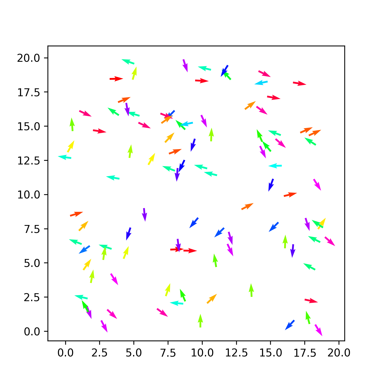
We can use matplotlib’s quiver plot to actually plot arrows.

def plot(conf,ax):
    qv = ax.quiver(conf["x"], conf["y"], conf["vx"], conf["vy"], conf["theta"], scale=1, scale_units='xy', cmap='hsv')
    plt.axis('equal')
    return qv

Combining all this together you should obtain something like the following

Visualisation of an initial configuration

Task 5: Python script to view the initial configuration

Embed the ideas above into your own pyvicsek.py file. you can run the script directly from the terminal with

python pyvicsek.py

Actual `Vicsek` dynamics

Now comes the actual challenge: we want to code the dynamics of the Vicsek model so that our updateRule() in System actually updates the positions and angles of the system.

Here was our algorithm after initialisation

Update rule

Neighbor Identification: For each particle \(i\), identify neighbors within radius \(r\).
Alignment: Compute the average direction of neighbors, including \(i\): \[ \bar{\theta}_i = \text{atan2}\left(\sum_{\rm j \in neighbours} \sin\theta_j, \sum_{\rm j \in neighbours} \cos\theta_j\right) \]
Noise: Add a random perturbation \(u\) to the orientation as a random variable uniformly distributed in the interval \([-\eta/2,\eta/2]\), where \(\eta\) is the noise strength

\[ \theta_i^{\text{new}} = \bar{\theta}_i + u \]
Update Position: Move each particle with its updated velocity: \[ \mathbf{r}_i^{\text{new}} = \mathbf{r}_i + \mathbf{v}_i \Delta t \]
Repeat: Iterate for the desired number of time steps.

There are a few central points:

we need to calculate all the updates before we apply them, otherwise the motion will not be synchronous
the calculation of the average local angle for alignment depends on sines and cosines. Directly averaging would be problematic (e.g. when two angles are close to \(+pi\) and \(-\pi\)).

The algorithm can be translated in pseudo-code.

Click to expand pseudocode

initialize new_theta array with size equal to number of particles

for each particle i:
    count = 10
    c, s = cos(theta[i]), sin(theta[i])
    for each particle j ≠ i:
        compute distance with periodic boundaries 
        if distance within interaction radius:
            accumulate cosine and sines of particle j in c, s
            increment count
    avg_theta = atan2(sin / count, cos / count)
    add uniform noise in [-pi, pi] to avg_theta and store in new_theta[i]

for each particle i:
    update position: 
        x += cos(new_theta[i]) * v * dt
        y += sin(new_theta[i]) * v * dt
    update orientation: 
        theta = new_theta[i]
    apply periodic boundaries to x and y

Task 6: Implement the dynamics

You can try and implement the pseudocode above or use the following snippet as a starting point. Complete the missing sections.

Then in, the main function in main.cpp, implement a for loop for a large number of iterations, were you repeatedly call the updateRule() member function and regularly save a configuration to a file with a new name.

To save a file with a new name, consider using C++ strings like

std::string root = "frame"
model.saveConfig( root+std::to_string(iteration));

Click to expand the snippet

void System::updateRule() {
    // Notice that "this" is not stricly needed for the member variables


    // COMPLETE THIS SECTION
    //correctly initialise new_theta as a vector of doubles.

    // get Lx and Ly values

    //END COMPLETE

    for (int i = 0; i < particleNumber; i++){

        int count = 1;

        // COMPLETE HERE
        // get cosine and sine of the angle of particle i
        double cos = std::cos(...);
        double sin = std::sin(...);
        
        for (int j = 0 ; j < particleNumber; j++){

            if (i!=j){
                // calculate distance
                double dx = particles[j].x - particles[i].x;
                double dy = particles[j].y - particles[i].y;

                // periodic boundaries
                if(dx>Lx*0.5) dx-=Lx;
                if(dx<-Lx*0.5) dx+=Lx;
                if(dy>Ly*0.5) dy-=Ly;
                if(dy<-Ly*0.5) dy+=Ly;
                
                // calculate the distance between the two particles
                double dist = std::sqrt(dx*dx + dy*dy);
            
                // check if the distance is below the interaction radius
                if (dist < particles[i].r){
                    // calculate the new orientation
                    cos +=  std::cos(particles[j].theta);
                    sin +=  std::sin(particles[j].theta);
                    count+=1;
                }
            }
        }
        
        //COMPLETE HERE
        // normalise sine and cosine to get the local average

        sin = ...;
        cos = ...;

        // average + noise
        double avg_theta = std::atan2(sin, cos);
        new_theta[i] = avg_theta + this->noiseStrength*this->uniform(-M_PI,M_PI);
    }
    // move the particles
    for (int i = 0; i < particleNumber; i++){
        particles[i].x += std::cos(new_theta[i])*particles[i].v*this->timeStep;
        // COMPLETE HERE
        // update also the y coordinate

        particles[i].theta = new_theta[i];
        // periodic boundaries
        if (particles[i].x >Lx) particles[i].x -= Lx;
        if (particles[i].x <0) particles[i].x += Lx;
        if (particles[i].y >Ly) particles[i].y -= Ly;
        if (particles[i].y <0) particles[i].y += Ly;
    }
}

Visualising the trajectory

Simple modifications to your Python code to include matplotlib’s Funcanimation allow you to visualise the trajectory

Here is a an example

import numpy as np
import matplotlib.pyplot as plt
import glob
import natsort
from matplotlib.animation import FuncAnimation

def read_config(filename, skip=2):
    """Reading an vicsek configuration from a file handle"""
    with open(filename, 'r') as file_handle:
        for i in range(skip): 
            next(file_handle)

        data = np.loadtxt(file_handle)
        conf = {}

        conf["id"] = data[:,0]
        conf["x"] = data[:,1]
        conf["y"] = data[:,2]
        conf["theta"] = data[:,3]
        conf["vx"] = np.cos(conf["theta"])
        conf["vy"] = np.sin(conf["theta"])  
        return conf

def plot(conf, ax):
    qv = ax.quiver(conf["x"], conf["y"], conf["vx"], conf["vy"], conf["theta"], scale=1, scale_units='xy', cmap='hsv')
    return qv

# files are stored in a folder
files = natsort.natsorted(glob.glob("frames/*"))

# first plot
fig, ax= plt.subplots() #

qv = plot(read_config(files[0]),ax)
plt.axis('equal')
plt.axis('off')

# function called to plot all files
def animate(i):
    print(i)
    conf = read_config(files[i])
    pos = np.array(list(zip(conf["x"], conf["y"])))
    print(pos)
    qv.set_offsets(pos)
    qv.set_UVC(conf["vx"], conf["vy"], conf["theta"])
    return qv,
    
# Create the animation
anim = FuncAnimation(fig,animate, range(len(files)))
# Show the animation
plt.show()

Task 7: View the trajectory

Adapt the script above to your setup and visualise your first trajectory!

Aims

Learning outcomes

Random initial state

Saving a configuration to file

Sprinkle some python: read the configuration a visualise it

Actual Vicsek dynamics

Visualising the trajectory

Sprinkle some `python`: read the configuration a visualise it

Actual `Vicsek` dynamics