Physics Challenge
This week, we’ll bring together the skills you’ve developed over the past four weeks to tackle a practical challenge. In this notebook, you’ll find a Physics coding challenge. This challenge is designed to consolidate your recent Python learning and give you practice working with strings, loops, and dictionaries.
Please Note: These challenges are designed to difficult! Do not worry if you are unable to complete a challenge in the time given. The important thing is that you are building resilience and practicing problem-solving skills - everything else is secondary!
Table of Contents
Background
Measuring Gravity with a Picket Fence and Photogate
A classic experiment in introductory physics is the photogate picket fence experiment. In this setup, a picket fence (a clear plastic strip with evenly spaced opaque bars) is dropped vertically through a photogate sensor.
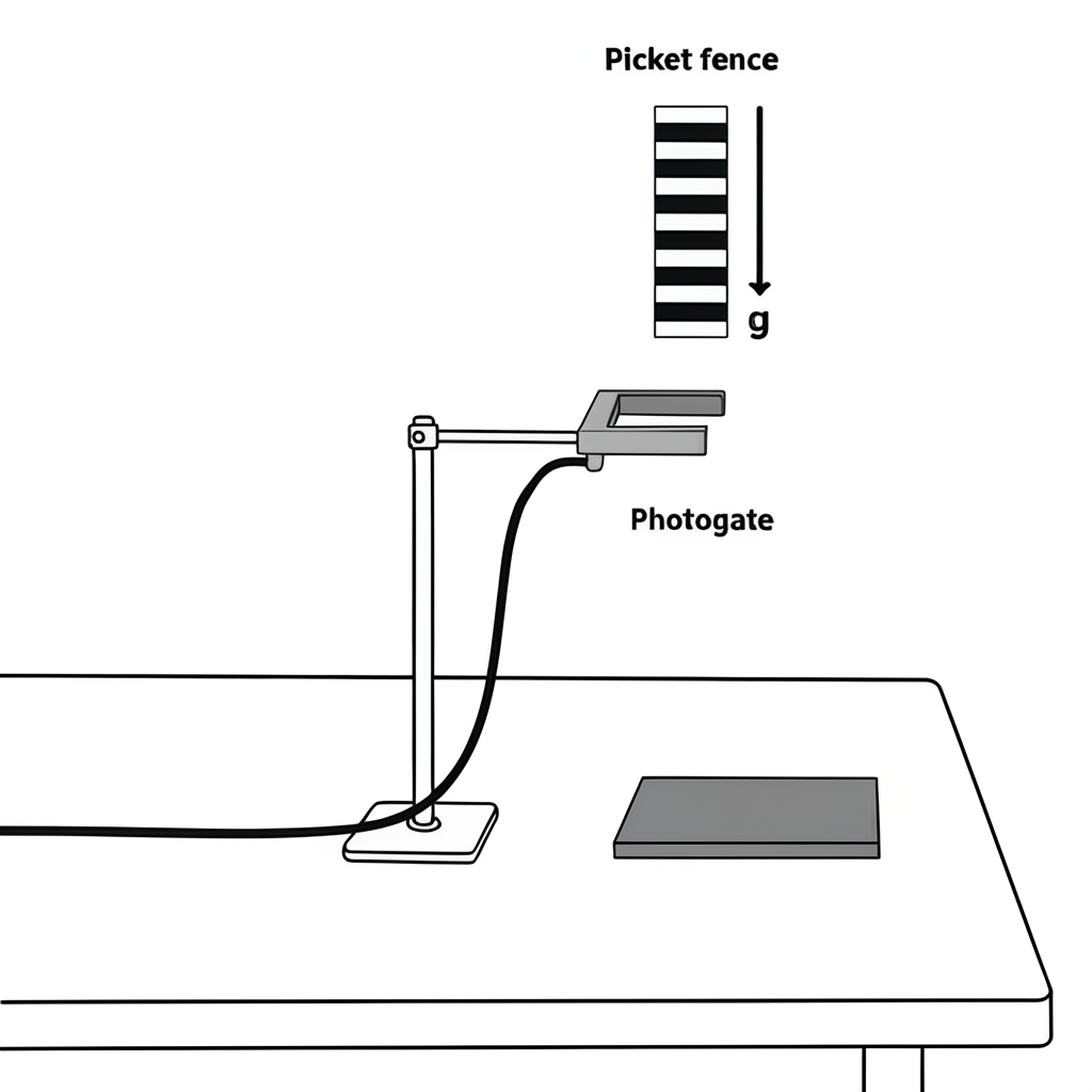
The photogate shines an infrared beam across a small gap. A sensor on the other side detects whether the beam makes it through or not. If the beam is blocked (by one of the bars), the sensor records 'x'. If the beam is not blocked, the sensor records 'o'. Every \(\Delta t = 0.5\) milliseconds (\(=0.0005s\)) the photogate logs whether the beam is blocked or not.
Because the bars on the picket fence are evenly spaced, the vertical distance between the start of one bar and the start of the next is always the same:
\[ \Delta d = 5 \text{cm (constant distance between bars).} \]
As the picket fence falls through the photogate, each bar successively blocks the beam. By measuring the time between when one bar starts blocking the beam and when the next bar does, we can estimate the velocity of the falling object. From changes in velocity, we can then estimate the acceleration due to gravity.
The Data
Note: Before starting this challenge, if you haven’t already, you may wish to read the sections on dictionaries in the week 1 intermediate notebook. This will be helpful in what follows.
You are given a Python dictionary that encodes \(100\) trials of the photogate picket fence experiment. Each entry:
- Has a key like
"Trial 1","Trial 2", … - Has a value that is a long string of
'o','x', and'e'characters, representing the sensor state at regular time intervals (recordings are taken \(\Delta t\) seconds apart). We can interpret these as follows:'x'= beam blocked (bar in photogate)'o'= beam unblocked (gap)'e'= error (the sensor glitched)
For example, suppose the dictionary contains the entry:
data_dict["Trial 1"] = "oooxxxoooxexo"This string represents the sensor readings for the first trial. Each character corresponds to a single timepoint, spaced by \(\Delta t = 0.0005\) s. We can interpret this as follows:
- The first three characters (
"ooo") mean the beam was unblocked at times \(t = 0 \text{ms}\), \(5 \text{ms}\), and \(10 \text{ms}\), - The next three characters (
"xxx") indicate the beam was blocked at \(t = 15 \text{ms}\), \(20 \text{ms}\), and \(25 \text{ms}\), - The next three (
"ooo") show the beam was unblocked again, - At \(t = 50 \text{ms}\), the character is
'e', indicating that the sensor glitched, - This is followed by
'x'and'o'at the final two timepoints.
Note: Across the \(100\) trials, several different picket fences were used. Some had the same number of bars, while others did not. Consequently, the number of black and white bars varied between trials.
The Challenge
Your challenge is to perform the following tasks:
Task 1: Clean the Data
Many trials contain one or more 'e' (error) characters due to sensor glitches. Apply the following rules to clean each string:
- If an
'e'(or group of'e's) is adjacent to at least one'x', replace all'e's in that group with'x', - Otherwise, replace them with
'o'.
For example, 'ooxexoeoxeeo' would become 'ooxxxoooxxxo'.
Task 2: Detect When Each Bar Begins to Block the Beam
Once the data is cleaned, your next task is to identify the exact times at which each bar starts to block the photogate beam.
This occurs every time the sensor reading transitions from 'o' (unblocked) to 'x' (blocked). Each from 'o' to 'x' transition corresponds to the leading edge of a bar entering the photogate.
To detect these moments:
- Loop through the cleaned string from left to right.
- Look for every index
iwhere the character is'x', and the character just before it (at indexi-1) is'o'. - For each such index, compute the time \(t = i × Δt\), where \(\Delta t =\) 0.5 milliseconds.
For each trial, you must save a list of timestamps (in seconds) showing when each bar starts to block the beam. For instance, given this cleaned string:
"oooxxxoooxxxooooxxx"You should detect transitions at indices: 3, 9, and 16 (remember, Python starts counting at 0!). In this case, the corresponding times would be:
[0.0015, 0.0045, 0.0080] # Computed by doing [3*0.0005,9*0.0005,16*0.0005]Task 3: Estimate Average Velocities
Once you’ve computed the times when each bar starts to block the beam, you can use those times to estimate the velocity of the falling picket fence.
From the previous, we have;
- \(\Delta d = 0.05\) meters is the constant distance between the leading edges of two consecutive bars.
- \(t_k\) and \(t_{k+1}\) are the times at which two consecutive bars start to block the beam.
We can now estimate the average velocity of the picket fence between two successive bar detections using:
\[ v_k = \frac{\Delta d}{t_{k+1} - t_k} \]
This gives the average velocity of the picket fence between the times \(t_k\) (when the \(k^{th}\) bar first blocks the sensor) and \(t_{k+1}\) (when the \((k+1)^{th}\) bar does the same).
For each trial, you must now use your list of bar-blocking times to compute a list of velocities between each pair of consecutive bars. For instance, if the bar-blocking times for a single trial are:
[0.0015, 0.0045, 0.0080]Then you must compute the velocities:
\[v_0= \frac{0.05}{0.0045-0.0015} = 16.66...\quad\text{and}\quad v_1= \frac{0.05}{0.0080-0.0045} = 14.28...\]
Task 4: Estimate Accelerations
Now that you’ve estimated velocities, you can use them to estimate how the instantaneous velocity of the picket fence changes over time - that is, its acceleration.
In step 3, each velocity \(v_k\) was calculated as an average over a time interval of the form \([t_k,t_{k+1}]\). We can treat this as a velocity recorded at the midpoint of the interval. That is, we treat this velocity as though it were recorded at the time \(\tau_k\), defined as:
\[ \tau_k := \frac{t_k + t_{k+1}}{2} \]
To estimate the acceleration between two consecutive velocities, we need to look at their differences. That is, we must compute:
\[ a_k = \frac{v_{k+1} - v_k}{\tau_{k+1} - \tau_k} \]
This gives an estimate of the average acceleration between the times \(\tau_k\) and \(\tau_{k+1}\). For each trial, you must now compute all such acceleration values, and then compute the average acceleration across the trial:
\[\overline{a}^{(j)} = \frac{1}{M_j} \sum_{k=1}^{M_j} a_k\] where \(M_j\) is the number of acceleration values in trial \(j\) (which is one less than the number of velocities).
Task 5: Estimate \(g\)
To obtain a final estimate of the gravitational acceleration, we must now average the acceleration values computed across all trials.
As in Step 4, let \(\overline{a}^{(j)}\) be the average acceleration for trial \(j\), and let \(N\) be the total number of trials. Then you must compute your final estimate of \(g\), given by:
\[ \hat{g} = \frac{1}{N} \sum_{j=1}^{N} \overline{a}^{(j)} \]
This value, \(\hat{g}\), represents your best overall estimate of the acceleration due to gravity based on the experimental data.