11  Macroscopic measurements

11.1 Introduction

In the course so far you have discussed the theoretical origins of phase transitions and have been given a theoretical introduction to the properties of disordered materials. In this section we will look briefly at some of the experimental techniques and experimental data that have driven and tested the theoretical work. Much of the quantitative experimental work is challenging and in many cases would take many lectures to justify properly. So, in these notes we will concentrate on the ideas underpinning the experiments and I will try to give a justification for the results obtained. The number of techniques discussed is limited and not exhaustive, you may find others as you read along.

11.2 Macroscopic observation and experiments

Before discussing experiments in detail it is worth taking a little time to think about our observation of phase transitions and the different types of material we encounter in our everyday life. In the following I will concentrate mainly on water and its states as we know them well. You may consider it as a liquid at room temperature, a solid at cold temperatures and a gas at high temperatures. However, even for this `simple’ material we can observe unusual effects as we change its state. So in the following I will use water as an example even though, hopefully, you can see how the ideas will apply in general to other materials.

11.2.1 1st Order Phase Transitions - ice and water as an example.

Phase transitions are all around us in our everyday life. Some take place naturally, for example, the freezing of water on a cold winter night, some are exploited (and maybe hidden) in the technology that surrounds us in for example, liquid crystal displays or non-volatile computer memory.

Let’s take water as our example and consider our everyday experience. In a warm building at a temperature of 20\(^o\)C, water in a beaker is a liquid, it freely flows and you can pour it from one container to another. What happens as we lower the temperature slowly (so that we keep, as best we can, a uniform temperature in the liquid). Common experience tells us it remains as a liquid until we reach its freezing point at 0\(^o\)C when it starts to solidify and form solid water - ice. But how does happen and does it always happen in the same way? Let’s think about this a little more deeply.

Suppose we put our beaker of water at 20\(^o\)C straight into a freezer at, say, -10\(^o\) C. To start with the water in the beaker will lose heat to the surroundings (mainly by conduction and convection) and temperature gradients will appear in the water (the water at the edges will be cooler than the water in the middle). As the outside approaches 0\(^o\)C we expect the water at the edges to freeze (we’ll discuss this further later) and a block of solid ice will eventually form in the beaker. (We might break our container as, unusually, the density of ice is less than water so the total volume occupied by the water tries to get larger). During this process we will have an ice-water \(\textit{interface}\) that stays at 0\(^o\)C but with large temperature gradients in the freezer and beaker - we are far from having the uniform temperature we mentioned above. As we can see from this short description, the temperature gradients mean that in practise phase transitions never take place uniformly in a material and there will always be some localization of the processes taking place. We can already see that freezing is more complicated than we might first imagine!

If we are going to look at the ice-water transition more carefully experimentally and to reduce these non-local effects we try to do things more slowly and try to maintain a uniform temperature by e.g. stirring. Ideally we’d also like to know qualitatively how quickly we are removing the heat and how much heat is removed in the process (the latent heat). What happens in this case? Well, if the outside temperature of the beaker is very slightly below zero then heat will be lost slowly from the (stirred) water and we expect small regions of ice mixed with the water to form. The water in the beaker does not freeze instantaneously but the ratio of the amount of ice to water steadily increases as heat is gradually removed (we should describe this as quasi-equilibrium where we consider we are moving gradually from one thermodynamic equilibrium state to another). As more ice forms we get a slushy mixture. If we carefully measure the temperature of the ice-water mixture (slush) during this process we will see that it remains at 0\(^o\)C until all the water has changed to ice at which point the ice will reach equilibrium with its surroundings (that we remember was just below zero). If, at any time during the process we prevent heat entering or leaving the system, the ice-water mixture will maintain the same ratio (although changes in the sizes of the regions may take place). The ice and water are then said to be in co-existence at the \(\textit{phase ~ transition ~temperature}\) of 0\(^o\)C.

Co-existence of two phases at the transition temperature is the typical characteristic of a first order transition.

You may wish to remind yourself of this process when we discuss thermal analysis later.

11.2.2 First Order transitions - Experimental measurements.

In the discussion above I tried to define more carefully how we were cooling the system. This hints at some of the difficulties in actually trying to measure the details of about what happens when the transition is taking place. Fundamentally we are trying to use equlibrium thermodynamics to explain what happens in a system that is not in equilibrium but in the process of equilibrating. The study of non-equilibrium processes is a very active and important area of study. We might note that the ice-water co-existence is an equilibrium state - it is all at 0\(^o\)C but can have very different appearances (slushy, an ice cube surrounded by water etc.). The result is that in all careful (accurate calorimetry) experiments care is taken to avoid non-unformity in the system (i.e. temperature gradients, field gradients in magnetic systems, …). The problem of non-uniform temeperature is even more acute for second order phases transitions as we will discuss below.

There are many ways in which you might study phase transitions apart from visually, but the most common, quantative and closely related techniques are Differential Thermal Analysis (DTA) and Differential Scanning Calorimetry (DSC). Machines for doing this are commercially available and are ubiquitous in materials science labs.

We will look at these techniques in more detail later.

11.2.3 First Order Phase transitions - nucleation and growth.

The form of the system after the transition has taken place may be of more interest for practical applications. For example, we know we can get ice by cooling water below 0\(^o\)C and if you are looking to cool your drink, the water in the form of a large ice cube is ideal (‘Scotch on the rocks’) whereas it wouldn’t be nice to ‘eat’ on a hot summers day. In contrast, if we can make ice crystals as small as possible (10’s of \(\mu\)m), we have the basis for making good ice cream. Indeed if the crystals are small enough the texture is creamy without the need for any ‘cream’ at all. Hence, the way in which macroscopic properties through the transition can be controlled may be as important as understanding the transition itself. For example, one favourite method of making ice cream is to use liquid nitrogen. This has the effect, with rapid stirring, of forming the tiny crystals needed for good ice cream. The processing of materials through phase transitions is ubiquitous. It’s perhaps no surprise to see that major industries including food processing, cosmetics, engineering materials are all heavily dependent on our knowledge of what happens as phase transitions take place.

To deepen our knowledge of how the transitions take place we need to think beyond the thermodynamics and ask what happens at the microscopic (atomic) level. So what happens to the atoms/particles as a first order freezing transition takes place? To make progress we need to introduce the ideas and theories of the nucleation and growth of crystals at the phase transition temperature. These concepts have been introduced in the theory part of these lectures but let’s thing about what happens in our water/ice system. If I start with liquid water at 0\(^o\)C and remove a small amount of heat from the system I expect, from our discussion above, to start forming an ice/water mixture. But how does the first ice crystal start to form?

The first thing to note and you may be surprised to learn is that crystallization doesn’t have to take place at all at 0\(^o\)C! It is perfectly possible to have stable liquid water below 0\(^o\)C even under standard atmosphere and pressure. This is known as supercooling or undercooling. It can also occur at other transitions, for example you can find superheated water above 100\(^o\)C. Although supercooled/superheated materials are not the equilbrium states they can stay in this \(\textit{metastable}\) state for many weeks/months on end unless disturbed.

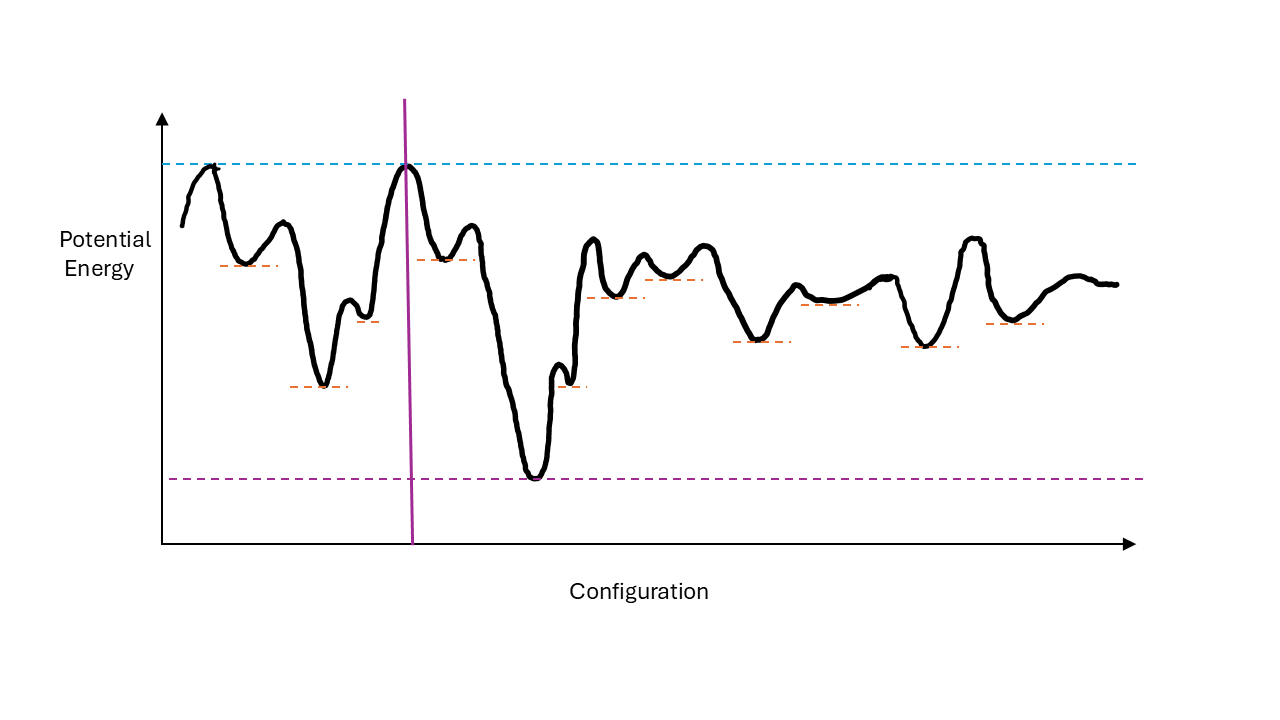
Hence, if we are careful we can cool water to well below 0\(^o\)C without it freezing. So what happens as we cool our water below 0\(^o\)C and why, in some cases does it not freeze? What observations measurements could we make? Firstly, if it supercools, no first-order phase transition has taken place and there is no release of latent heat. Hence, in heat capacity measurements (DSC) we would expect to see a steady and smooth decrease in temperature. The physical properties of the supercooled liquid water would stay broadly the same - it will still flow and pour as a liquid but we might observe steady changes in, for example, its volume or viscosity (which we will discuss in relation to the glass transition later) as the temperature decreases. But where has the heat (energy) associated with the latent heat of freezing (if the sample had frozen) gone? The answer is it hasn’t gone anywhere, it remains in the water even though the temperature has decreased. In other words there is more energy in supercooled water at -10 \(^o\)C than ice at the same temperature. Hence, the metastable state is not the \(\textit{global}\) minimum energy configuration of the system but is at a \(\textit{local}\) energy minimum (i.e. it will return to this local equilibrium after small deviations from the equilibrium state). In order for the global minimum to be reached from the local minimum there is an energy barrier to overcome. In order to freeze from the supercooled state this energy barrier needs to be overcome. The idea that there may be one or more possible local minima for a configuration is known as the \(\textit{energy landscape}\) of the material. This is illustrated conceptually in the figure below. Any configuration that lies above the landscape (the squiggly line) is a possible state of the system. For a given energy the system is rapidly changing configuration by moving to a neighbouring state on the configuration axis (in practise the energy landscape is multidimensional). At high energies (above the blue dotted line) it is possible to reach any configuration of the system in time. This would be equivalent to the normal liquid state. The lowest minimum (green dotted line) represents the equilibrium (minimum energy state) state e.g. ice. Now we imagine starting in the liquid state to the left of the vertical purple line and remove some energy. Once we are below this line we see that we cannot access any states to its right - the global minimum, ice, has become inaccessible. If we continue to remove energy we may find ourselves in the local minimum in this part of configuration space. This could perhaps be the supercooled liquid state. To reach the global minimum we have to overcome the energy barrier separating the local from the global minimum. Natural fluctuations in energy may be sufficient and explain why under normal cicumstances we get to the global minimum. However, if the local minimum is deep enough we get stuck in the metastable state.

In principle we could get ‘stuck’ in any of the local minima if we process our material in a certain way.

So what happens as we cool the water further - there are two possibilities: it will suddenly freeze to form ice (we find the global minimum energy), or its viscosity becomes so high that the internal molecular motion of the atoms is slowed down so much that the disordered arrangements of the atoms become ‘frozen’ so that it forms a ‘solid’ disordered structure that we call a glass (i.e. we’ve got stuck in a local minimum). In fact, no one has ever been able to produce ‘glassy’ water in this way \(^*\) but the transition to a glass on cooling does a occur in many materials. We’ll leave discussion of the glass transition and how we observe it until later.

So, if we observe our water as we cool it, we find it will suddenly and rapidly appear to freeze to form ice. If you seacrh for `supercooled water’ on youtube (or other) you will find many videos of this happening. So what is happening? In our supercooled water there will always be small regions that spontaneously start to form the atomic arrangements reminiscent of the crystal you’d expect to see at that temperature. But, as you’ve seen in the theory lectures, there is an energy barrier to overcome before the crystals become large enough to start growing continuously. In other words our embryonic crystals start to grow but dissolve again before they have the chance to grow further. However, if a crystal gets large enough, there is no energy barrier to stop more atoms/molecules attaching to the nascent crystal and it will continue to grow.

Once the crystals are macroscopically large we start to see them and can observe the growth. However, there are a few things we should note. Firstly, this spontaneous crystallization (known as \(\textit{homogeneous nucleation}\)), is a ‘local’ event - it could happen anywhere in the liquid. There are many questions that can then be asked. Is it only one crystal that forms and grows, or does homogeneous nucleation take place simultaneously in different parts of fluid at the same time? This poses some very difficult questions and when you investigate further you realise that the simple theory of nucleation and growth is just that - in reality how and where nucleation physically takes place in different materials is hard to predict! In some materials you might see a small number of large crystal form, in others, lots of smaller crystals start to form at the same time. In many cases you see a `front’ of nucleation advancing rapidly from the original nucleation event. We don’t have time in these lectures to explore this fascinating subject but the consequences for materials science (i.e the strength and physical properties of the materials produced) are important.

There are still a few things we should note. We know in our example that there is more energy in the supercooled liquid water than the same amount of water in the form of ice. So what happens when an ice crystal starts to grow spontaneously in our supercooled water? As the crystal starts to grow, the latent heat associated with the transition, that has remained in the liquid, must be released, so locally around the forming crystal the temperature of the liquid and the crystal will start to rise. In other words temperature gradients will start to form around the crystal and heat will only leave via transport processes (conduction, convection, possibly radiation) through the liquid. So, as the nucleation takes place the material is far from equlibrium with large variations in temperature present etc. What is the final state of the system once equlibrium has been reached in an isolated system? Well, as we noted, as nucleation takes place, the temperature goes up. So, do we end up with ice at a temperature below zero or a mixture of ice and water, which we know should be at 0\(^o\)C (at stp)? The answer is the latter, you end up with an ice/water mixture at 0\(^o\)C with the ratio of ice to water dependent on the level of supercooling. The more deeply supercooled the greater the proportion of ice to water.

Exercise. Look up the latent heat of freezing for water and estimate the temperature at which supercooled water needs to be if it was form only ice (i.e. no water) at 0\(^o\)C on nucleation.

From the discussion above you can see that the local and microscopic nature of the nucleation processes make precise experiments difficult. The results will depend, on the size of the sample, the rate of heat transfer through the sample, the randomness, of the nucleation processes, whether the process was at fixed pressure or constant volume (remember ice at stp has lower density than water and think about the implications if the process takes place at constant volume) etc.

So how does a first order transition from a supercooled state manifest itself in a calorimetry experiment, for example in a DSC? Well, if the transition takes place at the freezing temperature we’d expect to see the temperature of the sample remain at the transition temperature until the transition is complete, at which point the temperatures starts to drop steadily again at a rate corresponding to the heat capacity of the material. If however the material supercools its temperature will decrease steadily through the the transition temperature (no transition takes place). When the material eventually nucleates and crystallizes you observe a sudden rise in temperature (back to the transtion temperature) where it stays until the transition is complete and the temperature decreases as before. The deeper the supercooling the bigger the temperature jump. As noted above, the precise shape of the reheating peak observed depends on the sample size, thermal conductivity etc.

The sudden reheating of a material from a supercooled state is called \(\textit{recalescence}\).

Exercise. Recalescence is not confined to liquid/solid/gas transitions. It may occur for any first order transition, for example, the austenitic transition in stainless steel which is of commerical importance. Can you find other examples.

Final comments about 1st order phase transitions.

• Supercooling is often difficult to achieve. The reason is that in real situations we need to hold the material in containers in which there might be impurities or specks of dirt etc. These impurities can act very much like embryonic crystals that form in homogeneous nucleation and they lower the free energy barrier for nucleation. Processing materials under very clean conditions in smooth walled containers is very difficult. Nucleation on impurities is known as \(\textit{heterogeneous}\) nucleation and is often the process most observed unless great attention is taken to the preparation method.

• If there is a known transition and neither the transition or recalescence is observed in for example a DSC scan, then it is possible that the material formed a glass. This is discussed below.

\(^*\) Although it is possible to make amorphous ice - a topic great interest but we don’t have time to study it here.

11.2.4 Phase Separation in mixtures - spinodal decomposition.

In the previous section we saw that a first order transition doesn’t necessarily take place at the transition temperature. That is, rather than observing two phases in coexistence at the transition temperature, the material may remain in a metastable supercooled or superheated single state. The crucial observation is that for the transition to start, a nucleation event needs to take place, from which the second phase will grow. The next question you might ask is what happens if I continue to cool the material? Firstly, as the temperature difference increases the likelihood of homogeneous nucleation (and recalescence) increases. However, there are other possibilities, the material may form a glass (which we will discuss shortly) or we reach the point where spinodal decomposition takes place. You have discussed spinodal decomposition in the theoretical section of this course, but briefly there comes a point where the barrier to the separation disappears and the formation of two distinct phases occurs throughout the material (it does not rely on a nucleation centre). This is especially true if you are below and close to the critical point. This is a dynamic process as the size of the different regions grows over time - eventually two distinct macroscopically large phases appear. Spinodal decomposition, has an important role to play in material processing as it has an effect on the microsctructure of the material produced. If the material is quenched fast the growth of the separate regions that form will be rapidly arrested leading to a fine grained solid. If the quench is slow the resulting structure will be coarse grained. This graining of the microstructure will affect the physical properties of the material produced. This behaviour is most associated with phase transitions that involve the separation of components in composition, such as metallic alloys and polymer blends rather than pure liquid/gas, liquid/solid transitions in which spinodal decomposition is far harder to observe.

11.2.5 The Glass Transition.

In the section above we discussed how, particularly in the case of compositional phase separation, the microstucture of a material may be related to the speed in which it is quenched. As a consequence the end point is a material that is composed of a mixture of different phases rather than a single phase - the result of a true first order phase transition. So, what happens if we manage to cool without nucleation or spinodal decomposition occuring? i.e. what happens if we rapidly quench the sample to the extent that the dynamics driving for example spinodal decomposition are ‘frozen’ out. If we manage to slow the diffusion of the atoms enough, then the atomic re-arrangements needed to cause crystallization or spinodal decomposition cannot take place and the atoms/molecules appear to be fixed in place, but with a disordered arrangement. However we note that overall the material remains homogeneous and uniform - there is no microstructure. As in the case of supercooled liquids, this is not the equilibrium state, but another form of metastable state known as a glass. An example, is typically the material in our windows, `glass’, that is the result of cooling liquid silicates. Not all materials readily form glasses and this is often expressed loosely as the glass forming ability of the material. A good glass former is a material that can be cooled quite slowly, a poor glass former is one that needs to be quenched fast (there are more complex definitions but this is the gist). A characteristic of the glass is that no transition appears to take place in the material as it is quenched. There is no latent heat released, there is no recalescence and there is no evidence of phase separation (microstructure) in the material produced. In other words we imagine the glass forming from the supercooled liquid. So what do we mean by the glass transition and the glass transition temperature \(T_g\)? To answer this question, it is interesting to ask what happens as we heat our glass up? If, all we had was a very very high viscosity (behaving like a solid), but metastable supercooled liquid phase, then we would eventually return to the true liquid phase (above the melting point) without any evidence of a phase transition taking place (unless nucleation and recalescence took place). However, when we heat glass, we do see heat evolved at a temperature below the melting point (we’ll see this later on our summary of thermal analysis). For any given glass this occurs consistently at roughly the same temperature (but notably not well defined) and the material will start to change into a more viscous, `rubbery’ state. This is known as the glass transition. It is not a true thermodynamic transition and there are many ways in which it may defined (all occuring at roughly the same temperature). It depends on cooling/heating rate and can be observed in a change in for example viscosity, thermal expansion coefficients, heat capacity etc. It also depends on the thermal history of the material.

In summary, the existence of a glassy state of matter is readily apparent. However, the transformation of a liquid into a glass and how and why the structure changes on heating/cooling at the glass transition are still very poorly understood and the subject of much research. Indeed, there is no universal definition of the glass transition despite many attempts to define it in a rigorous thermodynamic way.

The terms glassy and amorphous materials are often used synonymously. Stricter definitions state that a (true) glass is formed by quenching from the liquid state whereas an amorphous solid includes materials that have been formed by for example deposition from a vapour, preciptation from a solution, mechanical processing. Amorphous materials also show a glass transition temperature but the manner in which they form is more complicated to describe theoretically.

11.2.6 Second Order Phase transitions

In the discussion above we charaterised a first order phase transtion as one in which latent heat is absorbed/emitted. i.e. one in which two phases coexist at the transition temperature and the temperature stays constant until the transition is complete. However, we can also identify other transitions in which no latent heat is associated with the change in phase taking place. Typical examples might be the liquid-vapour transition at the critical point or the ferromagnetic transition. The key point is that the transition between the two states is continuous. For example, in the ferromagnetic transition the magnetization is zero above the transition and increases steadily from zero below the transition. In this case it is the discontinuity in slope of the magnetization vs. temperature that is the signature of the transition taking place. In other cases a discontinuity in the gradient of the temperature dependence of the heat capacity is observed (while the heat capacity itself is continuous across the transition). These transitions have been discussed in the the theory section of this course and their beauty is the observation that the behaviour for a variety of supposedly very different physical transitions may be characterised in terms of universal behaviour. The \(\textit{universality class}\) of the transition is characterised by its critical exponents. You might note that many attempts have been made (unsuccessfully) to describe the glass transition in terms of an underlying second order phase transition.

Experiments to determine, for example, the critical exponents of the transition (rather than observing the transition itself) are extremely difficult. Precise control and accuracy of the temperature measurements is needed, great care must be taken to make any temperature gradients in the material as small as possible and in order to get accurate values of the critical exponents you need to get very close to the transition temperature.

12 Experimental observation of phase transitions

In the rest of this course we will highlight a few of the various techniques that are used to investigate and study the various forms of transitions discussed and the materials produced from them. Where possible we will relate them to some of the theoretical concepts that have been discussed in other parts. We will separate the discussion into four broad categories:

• observation of the changes in macroscopic variables associated with transitions,
• the structure and changes in structure in real space (i.e. positions of atoms and particles) as transitions take place,
• the structure and changes in structure as seen in reciprocal space (i.e. by scattering and diffraction),
• and the changes that take place in the structure and the dynamics of the particles in differennt phases.

12.1 Examples of macroscopic measurements.

12.1.1 Differential Thermal analysis.

Differential Thermal Analysis (DTA) methods are now a common and routine way of establishing the existenceo of phase transitions in materials in both a qualitative and quantitative way. The methods are all based on the same principle, namely the response to heating/cooling of the material under study is compared to that of a known calibration material that does not have any phase transitions in the region of study. I describe the two most common forms below.

12.1.1.1 Heat flux DSC (Boersma DTA)

This is the simplest thermal analysis technqiue. Two materials, a sample and a reference are heated together in a single furnace as shown below.

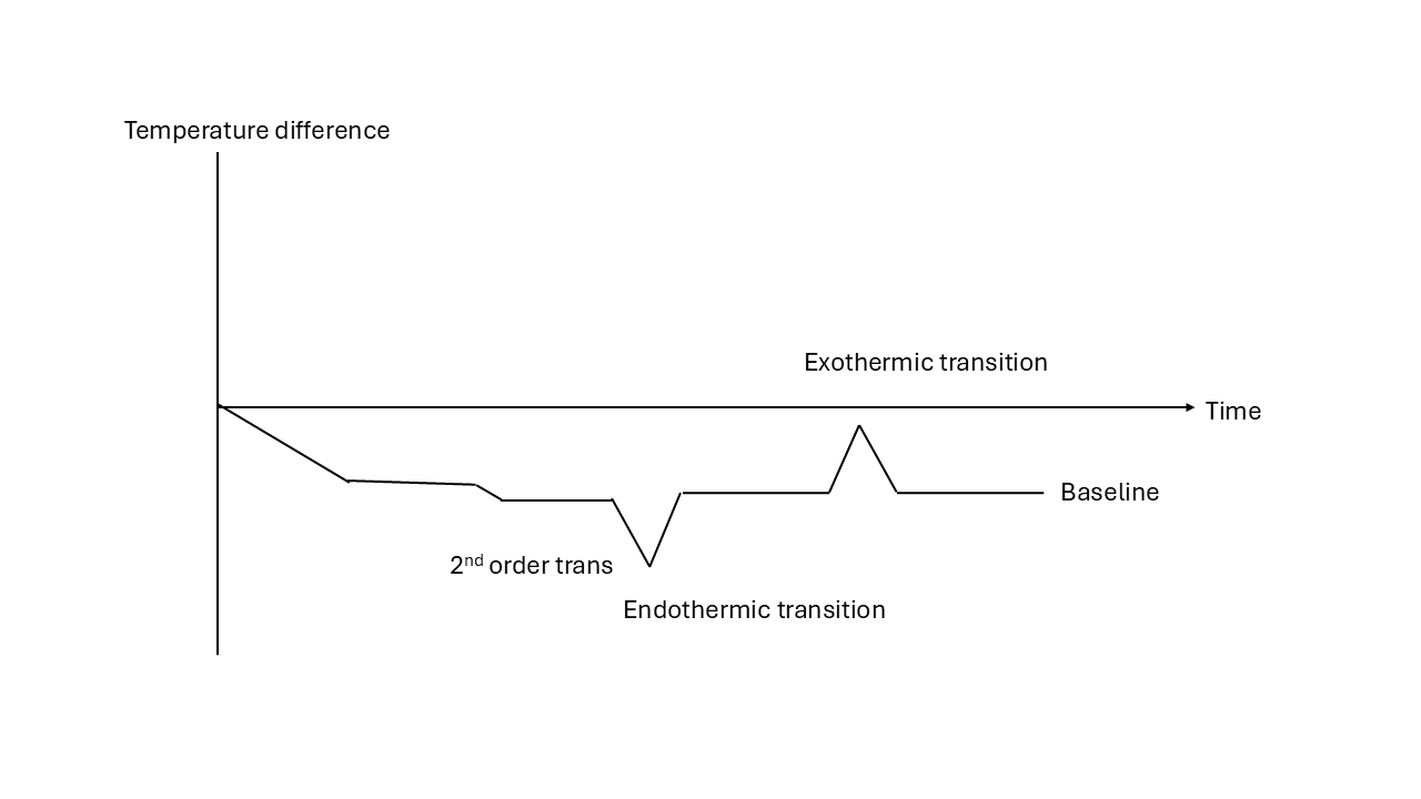
The temperature of the two materials is monitored carefully as the furnace is heated steadily. The reference is known not to show any phase transitions over the temperature range studied and will therefore heat steadily. If there is a phase change in the sample on heating/cooling, it will show as a temperature difference between the sample and reference. If the change is endothermic the sample will be at a lower temperature until the transition is complete after which the sample will catch up to the base temperature of the furnace, if the change is exothermic its temperature will increase until the transition is complete and then return to the furnace temperature. If the mass of the sample and reference is known and the heat capacity of the reference known, quantative values of, for example, latent heat, can be obtained. In quantitative measurements it is sometimes known as a heat flux DSC. A schematic of a heat flux DSC trace is shown below.

12.1.1.2 Heat flow DSC

This technique is similar to heat flux DSC but the sample and reference are located in their own separate furnaces (it is a double furnace technique). The power needed to steadily heat the sample and reference (and hence the heat added to the system) is controlled in such a way as to keep the temperature of the sample and reference the same.

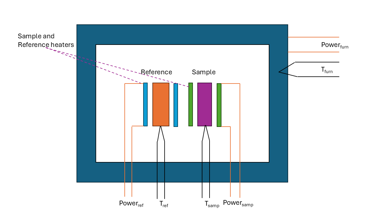
The difference in power supplied to the furnaces indicates when a transition takes place and with the mass of the reference and sample allows the energy absorbed/released in the transition be determined. If on heating there is a first order phase transition then more power is needed to overcome the latent heat to maintain the temperature. If an endothermic transition takes place then the power needed would decrease. The output from the instrument is usually presented as the heat flow to the sample as the temperature is raised. The trace is very similar in form to the heat flux DSC above except that the peaks and troughs observed are the opposite directions. (Increased heat flow into the sample is equivalent to the temperature of the sample being lower in the heat heat flux DSC). With computer control and a carefully designed and insulated chamber accurate measurements of latent heat etc. may be made.

12.1.1.3 Practical considerations

In use, practical questions involve the rate at which you wish to heat/cool the sample (transitions don’t take place instantaneously) and the sensitivity to small changes you are tryinh to observe. One common extension to the technique is \(\textit{Temperature ~ Modulated ~ DSC}\). In this case the heating/cooling may be modulated (e.g. stopped or reversed periodically. Application of this method allows the kinetics of the transition in the DSC to be observed. In particular, it can distinguish between a reversible second order phase transition and an irreversible transition such as the glass transition.

A typical DSC analysis would involve monitoring the sample as it is heated to some target temperature, for example, to above its melting point. (The limit would be set by the maximum temperature limit of the apparatus, the material stability (does it breakdown/oxidise) or the onset of a reaction between sample and container). If the sample was initially in a non equilibrium state (glassy, supercooled so you pass through \(T_g\) or recalescence takes place) then you do not expect to see transitions at the same place in the heating/cooling cycles. Similarly, observations of the differences in the DSC trace of materials with different thermal histories will be different.

12.1.2 Other techniques (non exhaustive)

Differential thermal analysis is not the only method for studying phase transitions. There are many other ways, quantitative and qualitative that may be used. Here are a few examples.

\(\bf{Thermal ~ mechanical ~ analysis ~ (TMA)}\). In this case the mechanical properties (modulus) of the material is observed on heating/cooling. For example, on heating, at the glass transition temperature, a glass will start to soften. Note, the glass transition temperature measured in this way is often slightly different to that measured by DSC and is indicative of the vagueness of the definition of \(T_g\) itself!

\(\bf{Thermogravimetric ~ analysis}\). Observation of changes in sample mass with temperature.

\(\bf{Imaging}\). It is quite possible to observe (and hence video) the phase transition taking place and getting some insight into the mechanism of the transition taking place.

\(\bf{Magnetic ~ susceptibilty}\). To observe transitions in para to ferro/antiferro magnetic transitions. (e.g. Curie and Néel points),

\(\bf{Electrical ~ Conductivity}\). In addition to structural changes in a material changes in other properties, for example, the electronic conductivity may also take place. For example, some chalcogenide (S,Se,Te) based materials are good glass formers and have very high resistivity (low conductivity) in the glassy state. By contrast, in the crystalline state they have high conductivity. The associated glass and melting transitions may be observed easily by measuring resistance. Indeed, the glass transition in these materials, is exploited in non-volatile memory devices.

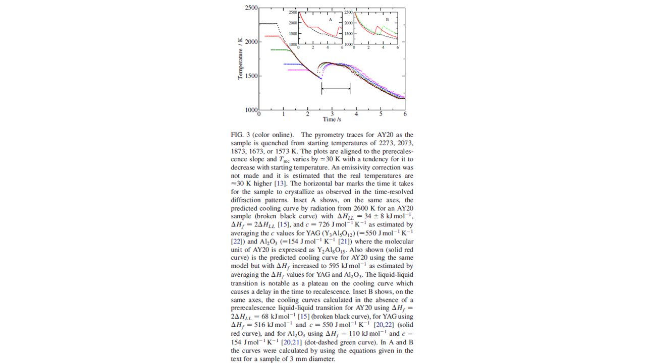
\(\bf{Pyrometric ~ measurements}\). This is an example from my own research on oxide glasses (that melt in excess of 2000K). In this case, the glass transition, recalescence, and freezing my all be observed in a semi-quantitative way by measuring the temperature of a cooling sample as a function of time.

12.2 Keypoints

We have taken some time here to discuss various aspects about phase transitions as macroscopically observable changes in a material. We have introduced the ideas of

• first and second order phase transitions,

• nucleation and growth,

• supercooling and superheating,

• spinodal decomposition,

• the formation of glasses

  andhave given a brief introduction as how to observe and measure them with especial emphasis on differential thermal analysis techniques.