5 Mean field theory and perturbation schemes
Of the wide variety of models of interest to the critical point theorist, the majority have shown themselves intractable to direct analytic (pen and paper) assault. In a very limited number of instances models have been solved exactly, yielding the phase coexistence parameters, critical exponents and the critical temperature. The 2-d spin-\(\frac{1}{2}\) Ising model is certainly the most celebrated such example, its principal critical exponents are found to be \(\beta=\frac{1}{8}, \nu=1, \gamma=\frac{7}{4}\). Its critical temperature is \(-2J/\ln(\sqrt{2}-1)\approx 2.269J\). Unfortunately such solutions rarely afford deep insight to the general framework of criticality although they do act as an invaluable test-bed for new and existing theories.
The inability to solve many models exactly often means that one must resort to approximations. One such approximation scheme is mean field theory.
5.1 Mean field solution of the Ising model
Let us look for a mean field expression for the free energy of the Ising model whose Hamiltonian is given in Equation 4.1 . Write
\[s_i=\langle s_i\rangle+(s_i-\langle s_i\rangle)=m+(s_i-m)=m+\delta s_i\]
Then \[\begin{aligned} {\cal H}_I=&-J\sum_{<i,j>}[m+(s_i-m)][m+(s_j-m)]-H\sum_i s_i\nonumber\\ =&-J\sum_{<i,j>}[m^2+m(s_i-m)+m(s_j-m)+\delta s_i\delta s_j]-H\sum_i s_i\nonumber\\ =&-J\sum_{i}(qms_i-qm^2/2)-H\sum_i s_i-J\sum_{<i,j>}\delta s_i\delta s_j \end{aligned} \tag{5.1}\] where in the last line we trnsformed from a sum over bonds to a sum over sites. Doing so makes use of the fact that when for each site \(i\) we perform the sum \(\sum_{<i,j>}\) over bonds of a quantity which is independent of \(s_j\), then the result is just the number of bonds per site times that quantity. Since the number of bonds on a lattice of \(N\) sites of coordination \(q\) is \(Nq/2\) (because each bond is shared between two sites), there are therefore \(q/2\) bonds per site.
Now the mean field approximation is to ignore the last term in the last line of Equation 5.1 giving the configurational energy as
\[ {\cal H}_{mf}=-\sum_{i}H_{mf}s_i+NqJm^2/2 \] with \(H_{mf}\equiv qJm+ H\) the “mean field” seen by spin \(s_i\). As all the spins are decoupled (independent) in this approximation we can write down the partition function, which follows by taking the partition function for a single spin (by summing the Boltzmann factor for \(s_i=\pm 1\)) and raising to the power \(N\) to find
\[ Z=e^{-\beta qJm^2N/2}[2\cosh(\beta(qJm+H))]^N \]
The free energy follows as
\[F(m)=NJqm^2/2-Nk_BT\ln[2\cosh(\beta (qJm+H)]\:.\]
and the magnetisation as
\[ m=-\frac{1}{N}\frac{\partial F}{\partial H}=\tanh(\beta(qJm+H)), \] where the first term drops out because we treat \(m\) as an independent variable when differentiating w.r.t. \(H\).
This is a self consistent equation because \(m\) appears on both the left and the right hand sides. To find \(m(H,T)\), we must numerically solve this last equation-self consistently. You will meet such an equation again later when you learn about mean field theories for liquid crystals.
In mean-field theory, the many-body interaction is replaced by an effective one-body problem in which each degree of freedom experiences an average field generated by all the others. The quantity that characterises the ordered phase—the order parameter—is precisely this average. Because the effective (mean-field) Hamiltonian is constructed using a presumed value of that average, internal consistency requires that the order parameter obtained by solving the effective problem match the value assumed to define it. Enforcing this equality yields a self-consistency condition for the order parameter. In practice: choose the effective field determined by the putative order parameter, compute the corresponding thermal average, and require that the two coincide.
Note that we can obtain \(m\) in a different way. Consider some arbitary spin, \(s_i\) say. Then this spin has an energy \({\cal H}_{mf}(s_i)\). Considering this energy for both cases \(s_i=\pm 1\) and the probability \(p(s_i)=e^{-\beta{\cal H}_{mf}(s_i)}/Z\) of each, we have that
\[\langle s_i\rangle=\sum_{s_i=\pm 1}s_ip(s_i)\] but for consistancy, \(\langle s_i\rangle=m\). Thus
\[ \begin{aligned} m & = \sum_{s_i=\pm 1}s_ip(s_i)\nonumber\\ \: & = \frac{e^{\beta(qJm+H)}-e^{-\beta(qJm+H)}} {e^{\beta(qJm+H)}+e^{-\beta(qJm+H)}}\nonumber\\ \: & = \tanh(\beta(qJm+H)) \end{aligned} \tag{5.2}\] as before.
5.2 Spontaneous symmetry breaking
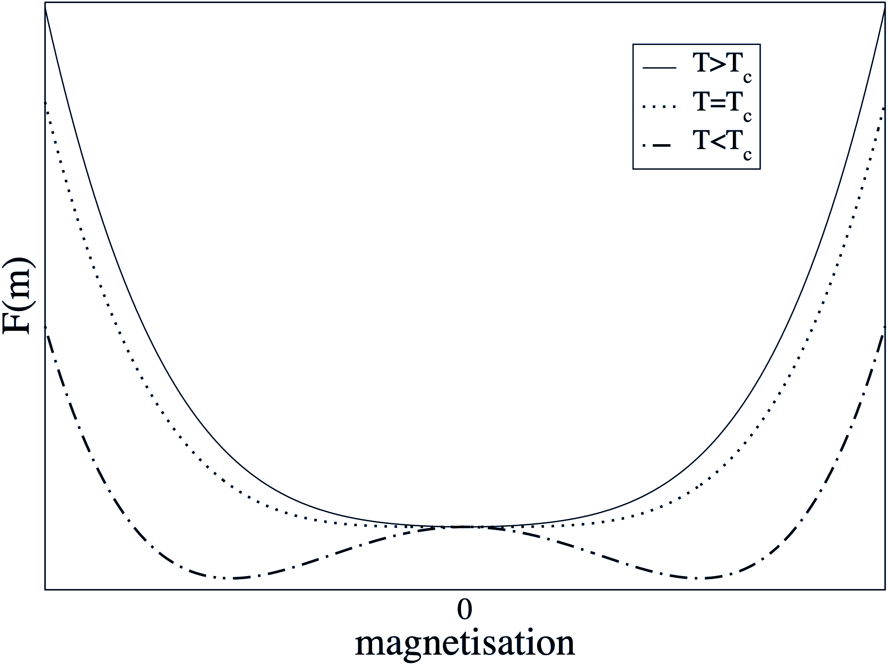
This mean field analysis reveals what is happening in the Ising model near the critical temperature \(T_c\). Figure 5.1 shows sketches for \(\beta F(m)/N\) as a function of temperature, where for f simplicity we restrict attention to \(H=0\). In this case \(F(m)\) is symmetric in \(m\), Moreover, at high \(T\), the entropy dominates and there is a single minimum in \(F(m)\) at \(m=0\). As \(T\) is lowered, there comes a point (\(T=T_c=qJ/k_B\)) where the curvature of \(F(m)\) at the origin changes sign; precisely at this point
\[\frac{\partial^2 F}{\partial m^2}=0.\] At lower temperature, there are instead two minima at nonzero \(m=\pm m^\star\), where the equilibrium magnetisation \(m^\star\) is the positive root (calculated explicitly below) of
\[m^\star=\tanh(\beta Jqm^\star)= \tanh(\frac{m^\star T_c}{T})\] The point \(m=0\) which remains a root of this equation, is clearly an unstable point for \(T<T_c\) (since \(F\) has a maximum there).
This is an example of spontaneous symmetry breaking. In the absence of an external field, the Hamiltonian (and therefore the free energy) is symmetric under \(m\to -m\). Accordingly, one might expect the actual state of the system to also show this symmetry. This is true at high temperature, but spontaneously breaks down at low ones. Instead there are a pair of ferromagnetic states (spins mostly up, or spins mostly down) which – by symmetry– have the same free energy, lower than the unmagnetized state.
5.3 Phase diagram
The resulting zero-field magnetisation curve \(m(T,H=0)\) looks like Figure 5.2.
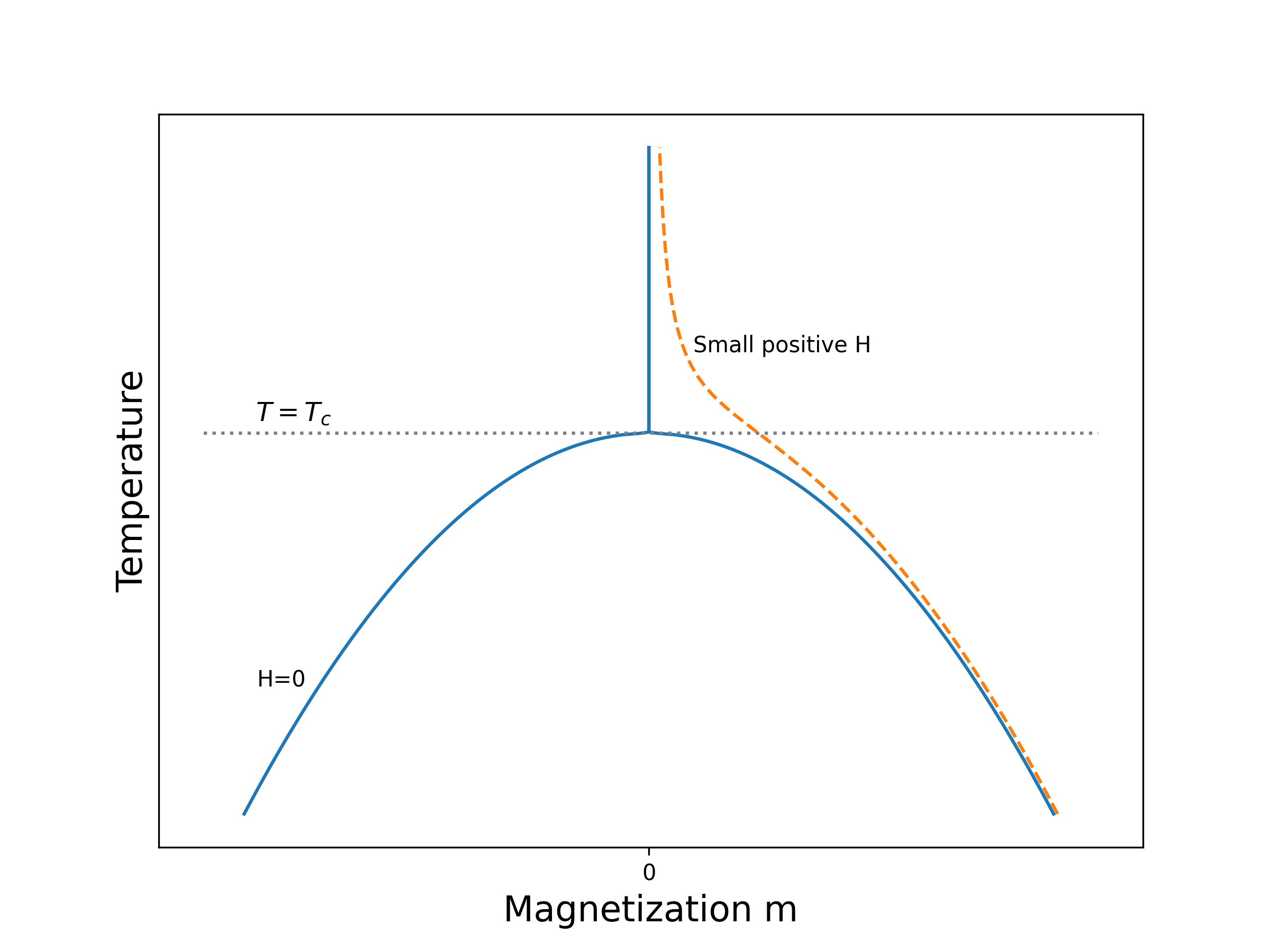
This shows the sudden change of behaviour at \(T_c\) (phase transition). For \(T<T_c\) it is arbitrary which of the two roots \(\pm m^\star\) is chosen; typically it will be different in different parts of the sample (giving macroscopic “magnetic domains”). But this behaviour with temperature is qualitatively modified by the presence of a field \(H\), however small. In that case, there is always a slight magnetization, even far above \(T_c\) and the curves becomes smoothed out, as shown. There is no doubt which root will be chosen, and no sudden change of the behaviour (no phase transition). Spontaneous symmetry breaking does not occur, because the symmetry is already broken by \(H\). (The curve \(F(m)\) is lopsided, rather than symmetrical about \(m=0\).)
On the other hand, if we sit below \(T_c\) in a positive field (say) and gradually reduce \(H\) through zero so that it becomes negative, there is a very sudden change of behaviour at \(h=0\): the equilibrium state jumps discontinuously from \(m=m^\star\) to \(m=-m^\star\).
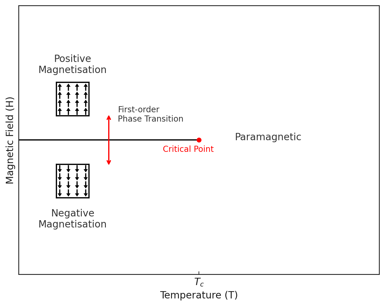
This is called a first order phase transition as opposed to the “second order” or continuous transition that occurs at \(T_c\) in zero field. The definitions are:
First order transition: magnetisation (or similar order parameter) depends discontinuously on a field variable (such as \(h\) or \(T\)).
Continuous transition (criticality): Change of functional form, but no discontinuity in \(m\); typically, however, \((\partial m/\partial T)_h\) (or similar) is either discontinuous, or diverges with an integrable singularity.
In this terminology, we can say that the phase diagram of the magnet in the \(H,T\) plane shows a line of first order phase transitions, terminating at a continuous transition, which is the critical point.
In some magnetic systems such as \(CePd_2Si_2\), one can, by applying pressure or altering the chemical composition, depress the critical temperature all the way to abolute zero! This may seem counterintuitive, after all at \(T=0\) one should expect perfect ordering, not the large fluctuations that accompany criticality. It turns out that the source of the fluctuations that drive the system critical is zero point motion associated with the Heisenberg uncertainty principle. Quantum criticality is a matter of ongoing active research, and open questions concern the nature of the phase diagrams and the relationship to superconductivity. Although the subject goes beyond the scope of this course, there is an accessible article here if you want to learn more.
5.4 A closer look: critical exponents
Let us now see how we can calculate critical exponents within the mean field approximation.
5.4.1 Zero H solution and the order parameter exponent
In zero field
\[m=\tanh(\frac{mT_c}{T})\] where \(T_c=qJ/k_B\) is the critical temperature at which \(m\) first goes to zero.
We look for a solution where \(m\) is small (\(\ll 1\)). Expanding the tanh function and replacing \(\beta=(k_BT)^{-1}\) yields
\[m=\frac{mT_c}{T}-\frac{1}{3}\left(\frac{mT_c}{T} \right)^3 +O(m^5)\:.\] Then \(m=0\) is one solution. The other solution is given by
\[m^2=3\left(\frac{T}{T_c} \right)^3\left(\frac{T_c}{T} -1\right)\]
Now, considering temperatures close to \(T_c\) to guarantee small \(m\), and employing the reduced temperature \(t=(T-T_c)/T_c\), one finds
\[m^2\simeq -3t\]
Hence
\[\begin{aligned} m= 0 & ~~~\textrm{for } T>T_c \:\:\: \textrm{since otherwise $m$ imaginary}\\ m= \pm\sqrt{-3t} & ~~\textrm{ for} \:\:\: T<T_c ~~\textrm{ real} \end{aligned} \tag{5.3}\] This result implies that (within the mean field approximation) the critical exponent \(\beta=1/2\).
5.4.2 Finite (but small) field solution: the susceptibility exponent
In a finite, but small field we can expand Equation 5.2 thus:
\[m=\frac{mT_c}{T}-\frac{1}{3}\left(\frac{mT_c}{T} \right)^3 +\frac{H}{kT}\]
Consider now the isothermal susceptibility
\[ \begin{aligned} \chi \equiv & \left(\frac{\partial m}{\partial H}\right)_T\\ = & \frac{T_c}{T}\chi - \left(\frac{T_c}{T}\right)^3 \chi m^2 + \frac{1}{k_BT} \end{aligned} \]
Then
\[\chi \left[ 1-\frac{T_c}{T} +\left(\frac{T_c}{T}\right)^3m^2 \right]=\frac{1}{k_BT}\]
Hence near \(T_c\)
\[\chi=\frac{1}{k_BT_c}\left(\frac{1}{t+m^2}\right)\]
Then using the results of Equation 5.3
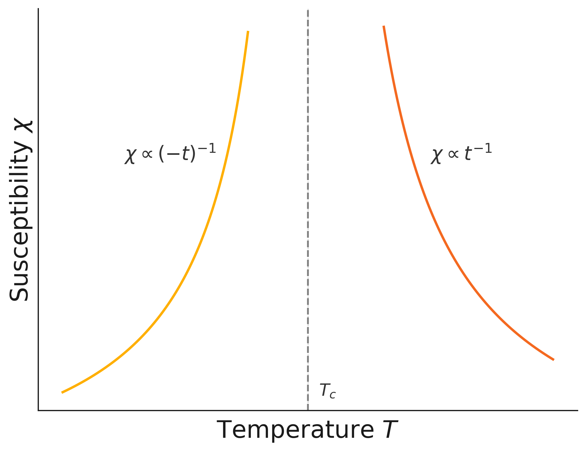
\[ \begin{aligned} \chi= (k_BT_ct)^{-1} & \textrm{ for} ~~~ T> T_c \\ \chi= (-2k_BT_ct)^{-1} & \textrm{ for} ~~~T \le T_c \end{aligned} \]
where one has to take the non-zero value for \(m\) below \(T_c\) to ensure +ve \(\chi\), i.e. thermodynamic stability. This result implies that (within the mean field approximation) the critical exponent \(\gamma=1\).
The schematic behaviour of the Ising order parameter and susceptibility are shown in Figure 5.5 (a) and (b) respectively.
5.5 Landau theory
Landau theory is a slightly more general type of mean field theory than that discussed in the previous subsection because it is not based on a particular microscopic model. Its starting point is the Helmholtz free energy, which Landau asserted can be written in terms of power series expansion of the order parameter \(\phi\):
\[ F_(\phi)=\sum_{i=0}^{\infty}a_i\phi^i \] The equilibrium value of \(\rho\) is that which minimises the Landau free energy.
We have already seen examples of these in earlier sections, e.g., for the liquid-gas transition this was \[ \rho_{liq} - \rho_{gas}: \quad \textrm{difference in density of two coexisting phases}, \] while for the Ising magnet it is the magnetisation \(m\). Both quantities vanish at the critical point. These are examples of scalar order parameters – a single number is required to represent the degree of order (\(n = 1\)).
In the absence of a symmetry-breaking field, the Landau free-energy density \(f_L\) must have symmetry \(f_L(-\phi) = f_L(\phi)\) (Ising case).
For some other systems, \(n\) component vectors are required in order to represent the order:
\[ \boldsymbol{\phi} = (\phi_1, \phi_2, \dots, \phi_n) \]
Then \(f_L(\boldsymbol{\phi})\) should be symmetric under \(O(n)\) rotations in \(n\)-component \(\phi\)-space.
The table below lists examples of order parameters for various physical systems.
| Physical System | Order Parameter \(\varphi\) | Symmetry Group |
|---|---|---|
| Uniaxial (Ising) ferromagnet | Magnetisation per spin, \(m\) | \(O(1)\) |
| Fluid (liquid-gas) | Density difference, \(\rho - \rho_c\) | \(O(1)\) |
| Liquid mixtures | Concentration difference, \(c - c_c\) | \(O(1)\) |
| Binary (AB) alloy (e.g., \(\beta\)-brass) | Concentration of one of the species, \(c\) | \(O(1)\) |
| Isotropic (vector) ferromagnet | \(n\)-component magnetisation, \(\mathbf{m} = (m_1, m_2, \dots, m_n)\) | \(O(n)\) |
| \(n = 2\): xy model | \(O(2)\) | |
| \(n = 3\): Heisenberg model | \(O(3)\) | |
| Superfluid He\(^4\) | Macroscopic condensate wavefunction, \(\Psi\) | \(O(2)\) |
| Superconductor (s-wave) | Macroscopic condensate wavefunction, \(\Psi\) | \(O(2)\) |
| Nematic liquid crystal | Orientational order, \(\langle P_2(\cos \theta)\rangle\) | |
| Smectic A liquid crystal | 1-dimensional periodic density | |
| Crystal | 3-dimensional periodic density |
Notes:
- In superfluid \(^4He\) the order parameter is
\[ \Psi = |\Psi| e^{i\theta}, \]
the complex wavefunction of the macroscopic condensate. Both the amplitude \(|\Psi|\) and phase \(\theta\) must be specified, so this corresponds to \(n = 2\).
Superconductors also correspond to \(n = 2\).
- In a nematic liquid crystal, the orientational order parameter is
\[ \langle P_2(\cos \theta) \rangle \equiv \frac{1}{2}\langle 3\cos^2 \theta - 1\rangle, \]
where \(\theta\) is the angle a molecule makes with the average direction of the long axes of the molecules (known as the director \(\hat{n}\)). Rotational symmetry is broken. For the case of an \(n\) component vector, the free energy should be a function of:
\[ \phi^2 \equiv |\boldsymbol{\phi}|^2 = \phi_1^2 + \phi_2^2 + \dots + \phi_n^2 = \sum_{i=1}^n \phi_i^2 \] in the absence of a symmetry breaking field. Rotational symmetry is incorporated into the theory.


To exemplify the approach, let us specialise to the case of a ferromagnet where \(\phi=m\), the magnetisation and write the Landau free energy as
\[ F(m)=F_0+a_2m^2+a_4m^4 \tag{5.4}\]
Here only the terms compatible with the order parameter symmetry are included in the expansion and we truncate the series at the 4th power because this is all that is necessary to yield the essential phenomenology. On symmetry grounds, the free energy of a ferromagnet should be invariant under a reversal of the sign of the magnetisation. Terms linear and cubic in \(m\) are not invariant under \(m\to -m\), and so do not feature.
One can understand how the Landau free energy can give rise to a critical point and coexistence values of the magnetisation, by plotting \(F(m)\) for various values of \(a_2\) with \(a_4\) assumed positive (which ensures that the magnetisation remains bounded). This is shown in the following movie:
The situation is qualitatively similar to that discussed in Section 5.2. Thermodynamics tells us that the system adopts the state of lowest free energy. From the movie, we see that for \(a_2>0\), the system will have \(m=0\), i.e. will be in the disordered (or paramagnetic) phase. For \(a_2<0\), the minimum in the free energy occurs at a finite value of \(m\), indicating that the ordered (ferromagnetic) phase is the stable one. In fact, the physical (up-down) spin symmetry built into \(F\) indicates that there are two equivalent stable states at \(m=\pm m^\star\). \(a_2=0\) corresponds to the critical point which marks the border between the ordered and disordered phases. Note that it is an inflexion point, so has \(\frac{d^2F}{dm^2}=0\).
Clearly \(a_2\) controls the deviation from the critical temperature, and accordingly we may write
\[a_2=\tilde{a_2} t\] where \(t\) is the reduced temperature. Thus we see that the trajectory of the minima as a function of \(a_2<0\) in the above movie effective traces out the coexistence curve in the \(m-T\) plane.
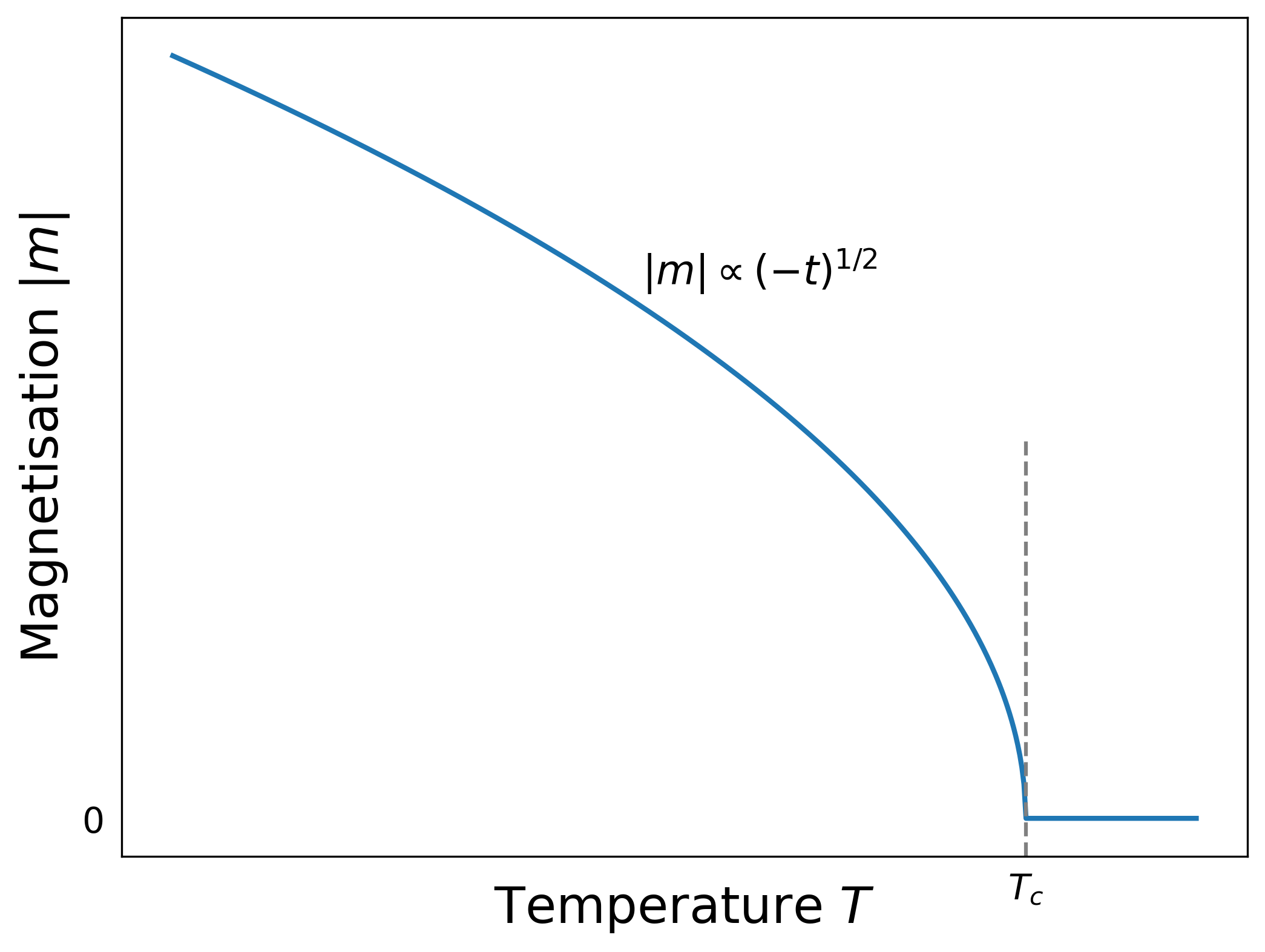
We can now attempt to calculate critical exponents. Restricting ourselves first to the magnetisation exponent \(\beta\) defined by \(m=t^\beta\), we first find the equilibrium magnetisation, corresponding to the minimum of the Landau free energy:
\[ \frac{dF}{dm}=2\tilde{a_2} tm+4a_4m^3=0 \tag{5.5}\]
which implies
\[m\propto (-t)^{1/2},\] so \(\beta=1/2\), which is again a mean field result.
Likewise we can calculate the effect of a small field \(H\) if we sit at the critical temperature \(T_c\). Since \(a_2=0\), we have
\[F(m)=F_0+a_4m^4-Hm\]
\[\frac{\partial F}{\partial m}=0 \Rightarrow m(H,T_c)=\left(\frac{H}{4a_4}\right)^{1/3}\]
or
\[H \sim m^\delta ~~~~~ \delta=3\] which defines a second critical exponent.
Note that at the critical point, a small applied field causes a very big increase in magnetisation; formally, \((\partial m/\partial H)_T\) is infinite at \(T=T_c\).
A third critical exponent can be defined from the magnetic susceptibility at zero field
\[\chi=\left(\frac{\partial m}{\partial H}\right)_{T,V} \sim |T-T_c|^{-\gamma}\]
Exercise: Show that the Landau expansion predicts \(\gamma=1\).
Finally we define a fourth critical exponent via the variation of the heat capacity (per site or per unit volume) \(C_H\), in fixed external field \(H=0\):
\[C_H \sim |T-T_c|^{-\alpha}\]
By convention, \(\alpha\) is defined to be positive for systems where there is a divergence of the heat capacity at the critical point (very often the case). The heat capacity can be calculated from
\[C_H =-T\frac{\partial^2 F}{\partial T^2}\]
From the minimization over \(m\) Equation 5.5 one finds (exercise: check this) \[ \begin{aligned} F = & 0 ~~~~T>T_c\nonumber\\ F = & -a_2^2/4a_4 ~~~~ T < T_c \end{aligned} \]
Using the fact that \(a_2\) varies linearly with \(T\), we have
\[ \begin{aligned} C_H =& 0 ~~~~ T\to T_c^+\nonumber\\ C_H =& \frac{T\tilde a_2^2}{2a_4} ~~~~ T \to T_c^-\:, \end{aligned} \]
which is actually a step discontinuity in specific heat. Since for positive \(\alpha\) the heat capacity is divergent, and for negative \(\alpha\) it is continuous, this behaviour formally corresponds to \(\alpha=0\)
5.6 Shortcomings of mean field theory
While mean field theories provide a useful route to understanding qualitatively the phenomenology of phase transitions, in real ferromagnets, as well as in more sophisticated theories, the critical exponents are not the simple fraction and integers found here. This failure of mean field theory to predict the correct exponents is of course traceable to their neglect of correlations. In later sections we shall start to take the first steps to including the effects of long range correlations.
| \(\:\) | Mean Field | \(d=1\) | \(d=2\) | \(d=3\) |
| Critical temperature \(k_BT/qJ\) | \(1\) | \(0\) | \(0.5673\) | \(0.754\) |
| Order parameter exponent \(\beta\) | \(\frac{1}{2}\) | - | \(\frac{1}{8}\) | \(0.325 \pm 0.001\) |
| Susceptibility exponent \(\gamma\) | \(1\) | \(\infty\) | \(\frac{7}{4}\) | \(1.24 \pm 0.001\) |
| Correlation length exponent \(\nu\) | \(\frac{1}{2}\) | \(\infty\) | \(1\) | \(0.63\pm 0.001\) |