PHYSM0071: First coursework assignment
1. Introduction and background
In this coursework assignment, you will explore the phenomena of spatial correlations and their relationship to phase behaviour in a simple lattice gas model. This model is a crude representation of a fluid in which particles can occupy the sites of a hypercubic lattice. The occupancy of a site \(i\) is specified by the variable \(c_i=1\) (occupied) or \(c_i=0\) vacant. The complete list of these occupancies \(\{c\}\) specifies a microstate. The instantaneous particle number density (fraction of occupied sites) is given by
\[ \rho=L^{-d}\sum_i c_i \]
where \(L\) is the linear extent of the lattice (i.e. the number of unit cells along a coordinate axis) and \(d\) its dimensionality.
Within the Grand Canonical ensemble (see precourse reading) the Hamiltonian of the lattice gas model is
\[{\cal H}_{LG}=-\epsilon\sum_{<i,j>}c_ic_j - \mu\sum_ic_i\]
where \(\epsilon\) is an attraction energy between a pair of particles on adjacent (nearest neighbouring) sites and \(\mu\) is a field known as the chemical potential which couples to the particle number density \(\rho\). The number density typically fluctuates around a mean value controlled by the prescribed value of \(\mu\).
One can also consider the model under conditions in which the particle number is fixed to some prescribed value - then there is no chemical potential and the corresponding set of microstates define the canonical ensemble (see precourse reading) of the lattice gas at that density.
1.1 Mapping between lattice gas and Ising model
The lattice gas model is interesting because whilst being a plausible model for a fluid, it maps onto the Ising model. We say that they are isomorphic to one another. This isomorphism extends the applicability of the Ising model. To expose the mapping we write the grand partition function of the lattice gas:
\[ \Xi=\sum_\textrm{ state}\exp-\beta{\cal H}_{LG}=\sum_{\{c\}}\exp\left[\beta \epsilon\sum_{<i,j>}c_ic_j +\beta\mu\sum_ic_i\right] \] where the sum runs over all possible combinations of occupancies of the lattice sites.
We now change variables to
\[c_i=(1+s_i)/2; ~~~~ J=\frac{\epsilon}{4}; ~~~~ h=\frac{\epsilon q+2\mu}{4}, \] where \(q\) is the lattice coordination number.
One finds,
\[{\cal H}_{LG}={\cal H}_\textrm{ I} + \textrm{ constant}\] Since the last term does not depend on the configuration, it feeds through as an additive constant in the free energy; and since all observables feature as derivatives of the free energy, the constant has no physical implications.
1.2 Phase diagram
Using the isomorphism we can plot the phase diagram of the lattice gas in the plane of average number density and temperature.
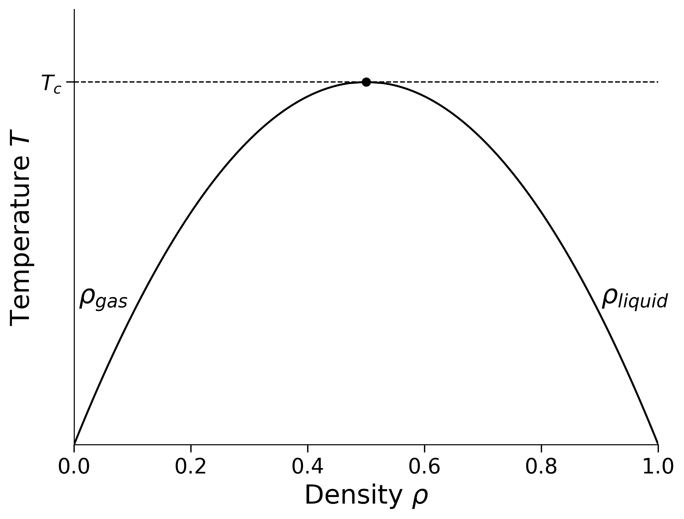
In the \(\mu-T\) plane there is a line of first order phase transitions terminating at a critical point which has density \(\rho_c=0.5\). The first order line means that if \(T<T_c\) and starting from the gas phase we smoothly increase the chemical potential through the coexistence value of \(\mu\), the average number density of particles on our lattice \(\rho=N/L^d\) jumps discontinuously from a low value \(\rho_\textrm{gas}\) to a high value \(\rho_\textrm{liquid}\). This is the gas-liquid phase transition. The values of \(\rho_\textrm{gas}\) and \(\rho_\textrm{liquid}\) merge at \(T_c\), the gas-liquid critical temperature. At higher temperatures, the distinction between the phases disappears.
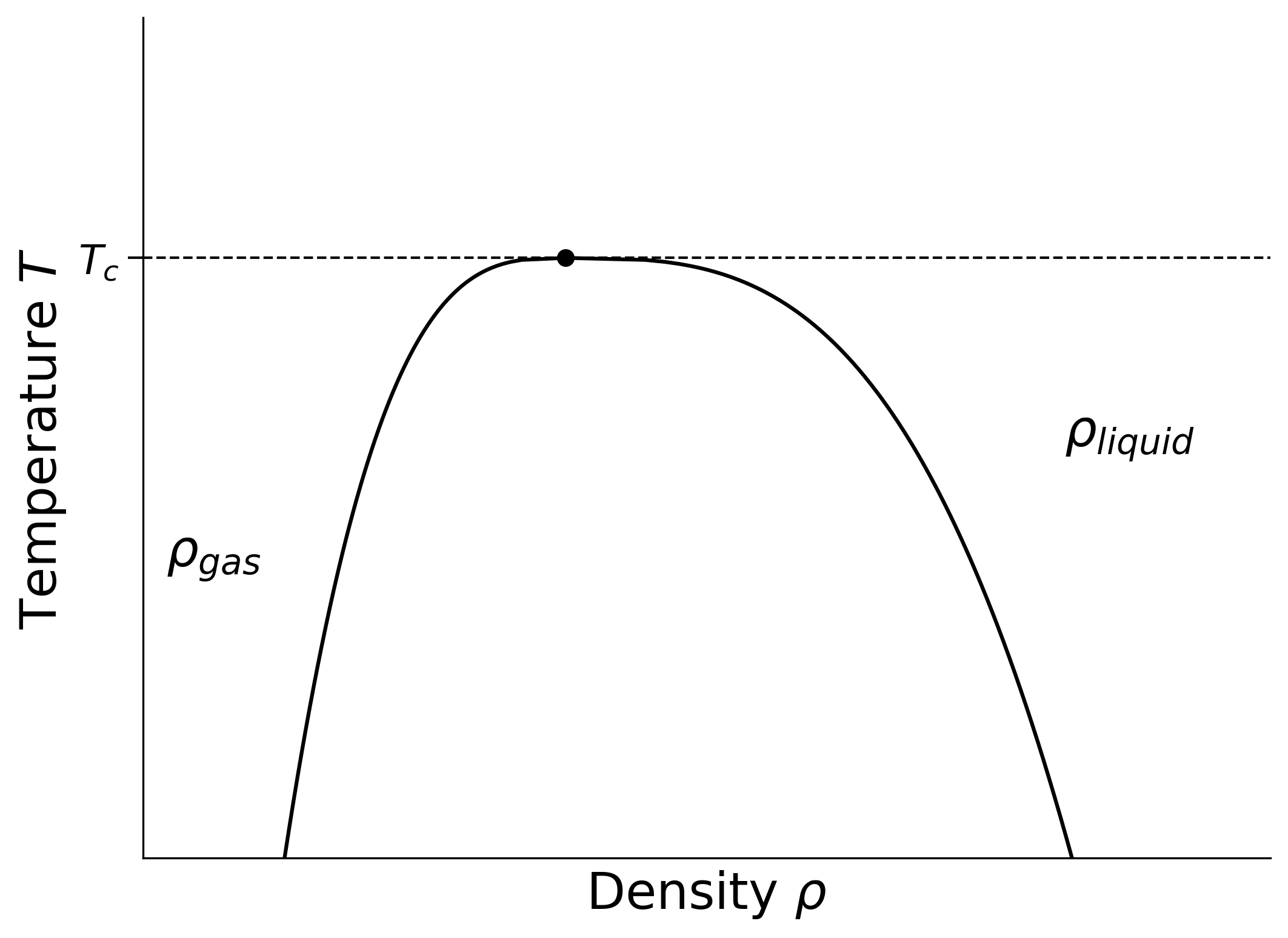
You may wish to compare the phase diagram of the lattice gas mode with the results of (say) van der Waals equation (see recommended textbooks for the required phase diagram). The main difference is that the lattice gas has so-called “particle-hole” symmetry, \(\rho\to 1-\rho\) (inherited from the up-down symmetry of the Ising model) which is not present for a real fluid. Accordingly, the phase diagram in a real fluid looks like a lopsided version of the above picture as shown in Figure 1.2. See here for some real experimental data showing the asymmetry of the coexistence curve in liquid metals.
2. Monte Carlo simulation
Monte Carlo methods are a class of algorithms that use repeated random sampling to obtain numerical solutions. For example, integrals can be approximated using Monte Carlo techniques by generating \({\cal N}\) random samples from the domain of integration \(A\) and evaluating the function at these points. For a 1D integral, the result is approximated as:
\[ I = \int_A dx \, f(x) \approx \frac{1}{{\cal N}} \sum_{i=1}^{{\cal N}} f(x_i), \]
where \(x_i\) are random points uniformly distributed in \(A\). In practice, while we cannot generate an infinite number of samples, using a large but finite \({\cal N}\) still provides a good approximation.
This idea also applies to sums over microstates, such as those appearing in the partition function of the lattice gas model. However, the space of all configurations is typically vast, and most configurations contribute negligibly to thermodynamic averages. Therefore, rather than sampling configurations uniformly, we use importance sampling, preferentially sampling microstates that contribute significantly to the ensemble.
In the grand canonical ensemble, the number of particles \(N\) is allowed to fluctuate, and importance sampling means that configurations are sampled with a probability proportional to the Boltzmann weight:
\[ P(C) \propto e^{-\beta [E(C) - \mu N(C)]}, \]
where \(E(C)\) is the energy of particle configuration \(C\), \(N(C)\) is the number of particles in that configuration, \(\mu\) is the chemical potential, and \(\beta = 1/k_BT\). To generate such configurations efficiently, one can use the Metropolis algorithm adapted for grand canonical importance sampling:
2.1 Grand Canonical Monte Carlo (GCMC) algorithm
A suitable algorithm for this case is to repeatedly update the system via the following fours steps:
Select a random lattice site \((i,j)\).
If the site is empty, propose inserting a particle. If it is occupied, propose removing the particle.
Compute the change in energy \(\Delta E\) and particle number \(\Delta N = \pm 1\).
Accept the move with probability:
\[ W(C \to C') = \begin{cases} 1 & \text{if } \Delta {\cal H}_{LG}< 0, \\ e^{-\beta \Delta {\cal H}_{LG}} & \text{otherwise}, \end{cases} \]
where \(\Delta {\cal H}_{LG} = \Delta E - \mu \Delta N\) is the change in the grand canonical Hamiltonian.
This update scheme allows the system to explore states with varying particle numbers according to grand canonical statistics.
2.2 Fixed-particle-number case (Canonical Ensemble)
In contrast, we may for simplicity want to simulate with the total number of particles \(N\) fixed, as in the canonical ensemble. Then particle insertions and deletions are not allowed and the chemical potential term drops out of the Hamiltonian. We can use Kawasaki dynamics, which conserves particle number by moving particles between lattice sites. An update consists of the following four steps.
Select two sites \((i,j)\) and \((i',j')\) at random.
If one site is occupied and the other is empty, propose exchanging the particle and vacancy.
Compute the energy change \(\Delta E = E(C') - E(C)\) associated with this proposed particle move.
Accept the move with probability:
\[ W(C \to C') = \begin{cases} 1 & \text{if } \Delta E < 0, \\ e^{-\beta \Delta E} & \text{otherwise}. \end{cases} \]
This approach ensures particle number is conserved while still allowing the system to explore equilibrium configurations of the canonical (ie. fixed \(N\)) ensemble.
2.3 Observables and measurement
A Monte Carlo sweep in either ensemble involves performing \(L^2\) update attempts on a lattice of size \(L \times L\).
The expectation value of a macrovariable \(O\) (e.g., energy, particle density, correlation functions) is estimated by averaging over sampled configurations:
\[ \overline O \approx \frac{1}{{\cal N}} \sum_{n=0}^{\cal N} O_n, \]
where \(O_n\) is the value measured in configuration \(C_n\), and \({\cal N}\) is the total number of configurations use for sampling.
Other observables (those which are second derivatives of the free energy) such as the heat capacity can’t be calculated as simple averages. Instead they are calculated as a variance. The formula for the specific heat capacity (cf. problem set) is
\[ C=\frac{1}{l^dk_BT^2} \left[\overline{E^2} - \overline{E}^2\right] = \frac{(\Delta E)^2}{L^dk_BT^2} \]
3. The assignment
You should investigate certain properties of the 2d square lattice gas model applying insight and knowledge from lectures and making use of a prewritten Python Monte Carlo code.
3.1 Setup
This should be completed in the week prior to the release of the assignment to make sure that any technical problems are resolved.
- On the PHYSM0071 Blackboard page open the Unit Information and Resources tab
- Scroll down to Notable and open it (if off campus make sure you have the UoB VPN enabled)
- Select the Jupyter Notebook (Legacy) notebook server option
- When the notebook has opened click the +Gitrepo button
- Under enter Git Repository insert: https://github.com/nbwilding/Lattice-gas-coursework
- Press the “clone” button. This will download a notebook called lattice-gas.ipynb into Jupyter
- Check that the program runs
- Familiarise yourself with the main features of the program. Pay attention to how to change the temperature, number of lattice sites \(N=L^2\), and the number of equilibration and sampling sweeps. Also check how to toggle live visualisation on and off. Be aware that the program can take several minutes to run depending on the system size, and equilibration/sampling parameters.
The assignment itself will be released at 12:30pm on Monday 13th October 2025 on Blackboard via the Unit Assessment tab. The submission deadline is Monday 27th October 2025 at 09:30.
Please contact me (nigel.wilding@bristol.ac.uk) if you have trouble with the setup described above, detailing the problem you encountered.
The various elements of the assignment are set out below. Instructions are given in italics.
3.2 Isomorphism of the lattice gas and Ising model
By referring to section 1.1 above, show that the Hamiltonian of the Lattice Gas model in the grand canonical ensemble
\[ {\cal H}_{LG}=-\epsilon\sum_{<i,j>}c_ic_j -\mu\sum_ic_i \] is transformed to that of the Ising model by means of the change of variable
\[ s_i=2c_i-1;~~~~ J=\frac{\epsilon}{4};~~~~ h=\frac{\epsilon q+2\mu}{4}. \] where \(q\) is the lattice coordination number (\(q=4\) in 2-dimensions and \(q=6\) in 3d). [4 marks]
Given that the critical temperature of the 2d Ising model is \(T_c\approx 2.269\: J/k_B\), use the above mapping to find the value of the critical temperature of the 2d lattice gas model in units of \(\epsilon/k_B\). [2 marks]
3.3 Code modification tasks
The program provided to you simulates the 2D lattice gas model in the canonical ensemble (i.e., at a fixed particle number density \(\rho\)), using the Kawasaki swap algorithm as described above. It allows the user to specify the number of lattice sites and the temperature for the simulation. The program computes the pair correlation function (also known as the radial distribution function) \(g(r)\) and the structure factor \(S(\mathbf{k})\) (refer to Chapter 2 of the notes for the definitions of these quantities).
In this implementation, the particle density is fixed at \(\rho = \rho_c = 0.5\). This choice ensures that the system approaches the critical point as the temperature is lowered within the supercritical regime. For convenience, the program uses dimensionless units by setting \(\epsilon = k_B = 1\). The linear system size is intially set to \(L=50\) lattice units.
Review the program thoroughly and gain a clear understanding of its functionality.
The program calculates the average form of the 2d structure factor \(S(\mathbf{k})\). Using this, obtain and plot an example of the radially averaged structure 1d factor \(S(|k|)\). [6 marks]
Add a function to calculate and print the dimensionless total energy and specific heat of the system. For the latter you will need the expression given in section 2.3, above.
[5 marks]
3.4 Computational investigations of correlations on the approach to criticality
Perform simulations at several (six or seven) temperatures within the super-critical range \(T_c \le T \lesssim 2T_c\). For each temperature, show the final configuration and describe how the overall structural characteristics evolve with temperature. Consider how you can be sure that your final configuration is equilibrated [4 marks]
Plot and compare the radial distribution function \(g(r)\) and the structure factor \(S(\mathbf{k})\), and its radially averaged form, \(S(|k|)\) at each temperature. [3 marks]
Interpret the peak structure in \(g(r)\) and \(S(|k|)\) and discuss the relationship to clustering or ordering. Interpret also the spikes in g(r). [4 marks]
The full width at half maximum (FWHM) of the radially averaged structure factor can be used to estimate the correlation length \(\xi\) through \(\xi= 1/FWHM\). For each temperature studied, estimate this quantity from your data. Plot the temperature dependence of \(\xi\) and comment on its behaviour. [4 marks]
3.5 Temperature and system size dependence of the specific heat
Examine how the specific heat capacity varies with dimensionless temperature over a broad range, including both subcritical and supercritical regimes (e.g \(T_c/2<T<2T_c\)). Plot and describe the overall behavior of the specific heat across this temperature range and offer an explanation for its form. Describe how you checked that your sampling was from reasonably well equilibrated configurations. [4 marks]
Repeat the analysis that you performed for the \(L=50\) system, for system sizes \(L=20\) and \(L=35\). Calculate error bars for all data point, describing how you did this. Compare the results for all three system size and highlight any observed differences. Discuss possible explanations for these size-dependent effects. [4 marks]
4.0 Your report
You should produce a short skeleton report (upto 4 sides of A4 including figures and in no less than 11 pt fontsize) focussing on and summarising the results of the above investigations and your comments/observations on the findings.
As well as a title and your name, the report should be laid out using the headings above:
- Isomorphism of the lattice gas and Ising model
- Code modifications. Include snippets of your modified code, highlighting the modifications in yellow. Do not include the whole code, just enough to see what you changed and where you did it.
- Computational investigations of correlations on the approach to criticality
- Temperature and system size dependence of the specific heat
- Include a line with following declaration at the end of the report: “I have not made use of Artificial Intelligence tools in completing this assessement beyond those of category 2 in the University’s categorisation scheme.”
There is no need for any other section headings ie. you don’t need abstract, introduction, references etc. Marks will be deducted for reports that exceed four sides (faces) of A4.
Submit your report in pdf format for grading via blackboard. The report will be marked out of 40, and will count for \(30\%\) of the unit mark.
Like any lab report, the marking focus will be on:
- Do your results look physically plausible?
- Did you describe the pertinent features?
- Are your descriptions clear?
- Do you explain them correctly using appropriate concepts?