12 Measurements in real space
In the theory part of the course you have been introduced formally to the radial distribution function \(g(r)\) and seen how it is a useful description of the arrangement of particles in a disordered system. In particular, in the absence of the long range periodic order that is associated with crystalline materials it is one of the first things we wish to find for liquid or glassy material. In our examples we assume that we are looking at a uniform and isotropic material, that is, there is no preferred direction in the material and no density variations on length scales much greater than the particle size. That is, macroscopically the material appears is of uniform density. It is also possible to give a more general definition \(g(\bf{r})\) where we recognise that there is some preferred orientation of the atoms around each other in the material but we will not consider it here.
12.1 A simple description of \(g(r)\)
In layman’s terms the radial distribution function is often described loosely as the probability of finding another particle at a distance from a particle at the origin. If we think about it this way we must remember that \(g(r)\) is a statistical function so what we are really trying to express is the average of this distribution taking each atom in the material in turn as the ‘origin’. Expressed in this way you might worry about what this means for atoms on the ‘edge’. Normally this is not a concern for large samples, but beware about the definition of \(g(r)\)if you start approaching ‘nano-sized’ materials.
A better definition is that \(g(r)\) represents the deviation from the mean particle density, normalised to one, as you move outward from a particle at the origin. At large \(r\) we expect this to equate to a constant, related to the mean particle density of the material. When properly normalised to the mean density \(g(r) _{r\rightarrow \infty} \rightarrow 1\). The figure below shows the key features of a typical radial distribution function.
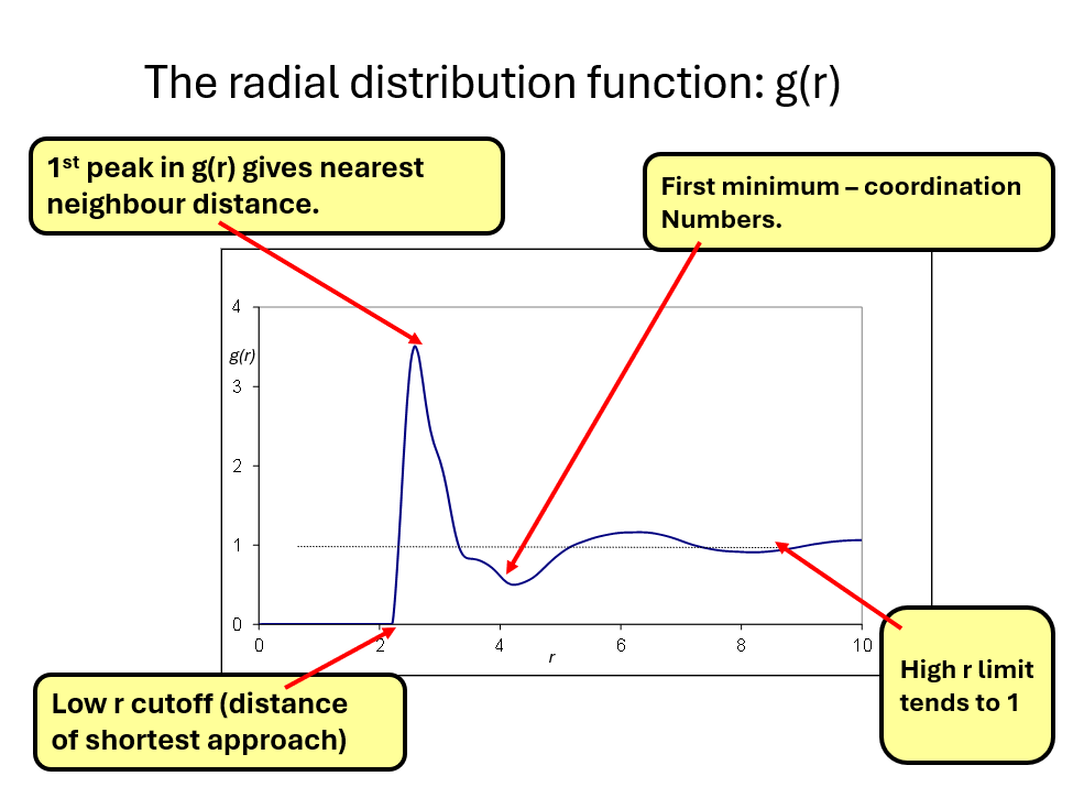
Points to note are
- that \(g(r) = 0\) for a distance below a ‘cutoff’ distance. This recognises that our particles have a finite size and when we mean ‘position of particle’ we mean its centre. Hence this cut off represents the diameter of the particles. What we mean by diameter of particle and what this means for \(g(r)\) we will discuss shortly.
- \(g(r)\) typically rises from 0 to give a ‘first peak’. The position of this peak is referred to as the nearest neighbour distance. (NB. it is not the same as the diameter of the particles).
- After the nearest neighbour peak, \(g(r)\) typically dips below the mean density and is characterised by damped oscillating peaks and troughs until \(g(r)\) reaches the constant mean density.
12.2 What can we learn from \(g(r)\)?
12.2.1 Peak positions.
The peaks observed in \(g(r)\) correspond to the most common interparticle seperation. For an atomic system, they can typically be associated with chemical bonds and as you move further in \(r\) the \(\textit{medium}\) (i.e. next nearest neighbour …) range ordering. However, we must remember that this is only a pair corrrelation function. It does not \(\it{per~se}\) tell us about for example bond angles. These are formally be obtained from higher order correlation functionz (triplet, …) but these are not obtainable directly from \(g(r)\) itself.
Note. If we have a crystalline material the peaks in \(g(r)\) will be narrow (they will have an intrinsic width at least due to thermal vibration) and at low values of \(r\), \(g(r)\) will be zero between them. However, even in a crystalline material these peaks will start to broaden and get smaller at high \(r\) until, again, \(g(r)\) reaches mean density.
12.2.2 Coordination numbers.
\(g(r)\) is a dimensionless function that normalises to a mean density of one at large \(r\). For a material with a \(\textit{number~density}\), \(\rho_N\), the mean number density at distance \(r\) is hence \(\rho_N g(r)\). A thin spherical shell of thickness \(\Delta r\) at a distance \(r\) will have a volume \(4\pi r^2 \Delta r\) so that the mean number of atoms in the shell will be,
\(4\pi r^2 \rho_N(r) \Delta r\).
Hence the mean number of atoms in a spherical shell of inner radius \(r_1\) and outer radius \(r_2\) will be given by,
\(\bar{n} = 4\pi\rho_N\int_{r1}^{r2}r^2g(r)dr\).
If we define a peak in \(g(r)\) by \(r_1\) and \(r_2\) we call \(n\) the coordination number of the particles in the peak.
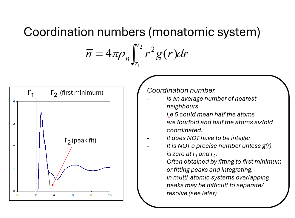
It is important to note that the coordination number is an average (\(g(r)\) is a statistical distribution) and in general will vary particle by particle in the material. It does not have to be integer and unless \(g(r_1)=g(r_2)=0\) it is an ill defined quantity. Nevertheless, it is a commonly quoted number in research papers so it is important to read carefully how it has been caclulated to obtain meaningful conclusions that can be compared to figures in other research work.
12.3 How to we measure \(g(r)\) directly for a material?
In order to measure \(g(r)\) directly, we need to obtain a 3D (unless we are looking at a 2D system) image of the material in which all the particle coordinates \(r_i(x,y,z)\) can be obtained. Although some modern techniques can obtain images with atomic resolution (for example scanning tunneling microscopy) they are mostly limited to surface imaging and not suitable for studying liquids (where atoms are moving around). Although some X-ray and electron microscopy techniques (see for example ptychography) can produce atomic scale resolution (using coherent imgaing techniques) these are again largely confined to 2D surfaces and are again not suitable for atomic liquids.
Historically (1950-60s) the first attempts to determine \(g(r)\) came from measurement of the packing of real particles made by literally constructing disordered structures with balls and sticks, gelatine balls, plasticine etc. and then painstakingly finding the particle coordinates during a careful and systematic disassembly. Needless to say this wasn’t a particularly accurate method but it did reveal, what suprised many at the time, dense packing of particles in liquids was characterised by 5-fold coordination.
Today there is much literature on the study of disorder and phase changes in colloidal systems (particles of the order of 100s of nanometres in size and greater) and we will take a look at some of the methods used to do these experiments. The spirit of these experiments is the same - we try to measure the positions of the particles in space and ideally also over time (to see how they move).
12.4 The structure of colloidal systems.
Colloids are complex systems composed of mesoscopic particles suspended in a host liquid. They and emulsions (liquid drops in a host liquid) are found everywhere around us. They are used extensively in food processing and paints etc. Much work has been done to stabilize and control their properties but here we will look briefly at how they have been used to study phase transitions, glasses and particle coordination in ‘simple’ systems.
In its simplest form a colloid consists of small (mesoscopic) particles suspended in a solvent. However, if you simply mix and stir say small spherical particles in a solvent you will often observe \(\textit{flocculation}\). Fundamentally, there is an attractive force, called the depletion force, that is driven by the excluded volumes (and associated entropy) around hard spheres as they come into contact. That is, the particles tend to clump together into larger aggregates. So, in order to produce a homogeneous phase of uniform particle density, the colloid needs to be \(\textit{stabilised}\). The stabilization of colloids and emulsions is a vast subject, but in short, by adding additional chemicals (e.g. surfactants) to the solvent it is possible to introduce some repulsion between the particles that overcomes the tendency to flocculate. The type and concentration of the added chemicals causes a change in the electrostatic attraction/repulsion between the particles and gives rise to the zeta (\(\zeta\)) potential. To mimic ideal `hard sphere’ behaviour the aim is to have a colloid with a zeta potential of zero. i.e. there is no net attraction or repulsion (except the hard sphere surface itself) between the particles.
There are other ways to stabilize colloids for example, steric repulsion. In this method long chain molelcules are incorporated into the particles to make them `hairy’. The presence of these hairs reduces the excluded volume around the particles and hence reduces the depletion force between them.
From here on we will assume that we are able to create such an ideal hard sphere colloid! For a comphrensive and detailed review of studies of colloidal hard sphere systems see the review of Royall et. al. 2024
12.5 How to we obtain \(g(r)\) and information about coordination from colloid systems.
If we have our ideal colloid there are several things we may wish to control. For example, what is the size of the particles (there will be a tendency for large particles to sediment), are the particles all the same size (polydispersivity), can we make systems with different shapes (e.g. ovoid), can we make systems with mixed particle sizes, can we introduce directional interactions (Janus particles) and how do you control the number density of the particles (the density of the particles is the crucial parameter for describing the hard sphere phase diagram)? These all pose theoretical and experimental difficulties of their own. Finally, once we’ve prepared our colloid with a controlled density … how do we study its structure (and dynamics)?
12.6 Confocal microscopy.
There are a few further steps we need to achieve to be able to measure and track the positions of the particles in our hard sphere colloid. Firstly, it is important that the particles are transparent, otherwise, we will not be able to see into the depth of the sample and secondly we need to match, as closely as possible, the refractive index of the solvent. If we don’t do this the difference in refractive index will mean light is quickly scattered in all directions meaning we will just have an opaque material. However, by making the particles all but invisible how to we determine their positions? The trick is to include a fluorescent dye their centre. When illuminated with the correct wavelength of light (using a laser) the particles will glow. This works well but how do we measure the positions of the particles in 3D. The answer is to use a confocal microscope as illustrated below (figure take from Royall et. al.2024).
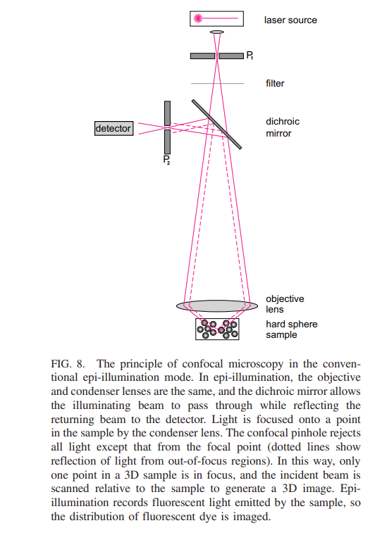
Note, moving the sample up and down changes the ‘z’ direction and a three dimensional image may be obtained by ‘stacking’ vertically scanned 2D images.
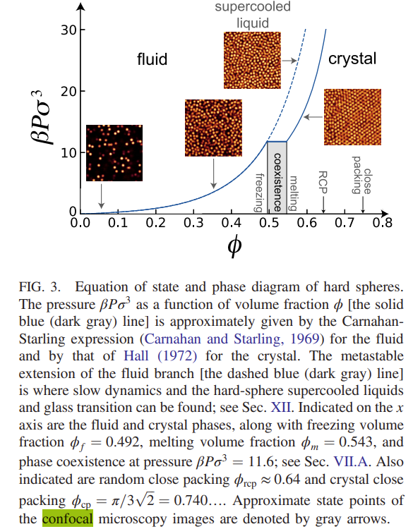
Once the particles positions have been determined it is possible to plot \(g(r)\) for the different packing densities to show how it varies over the phase diagram as shown below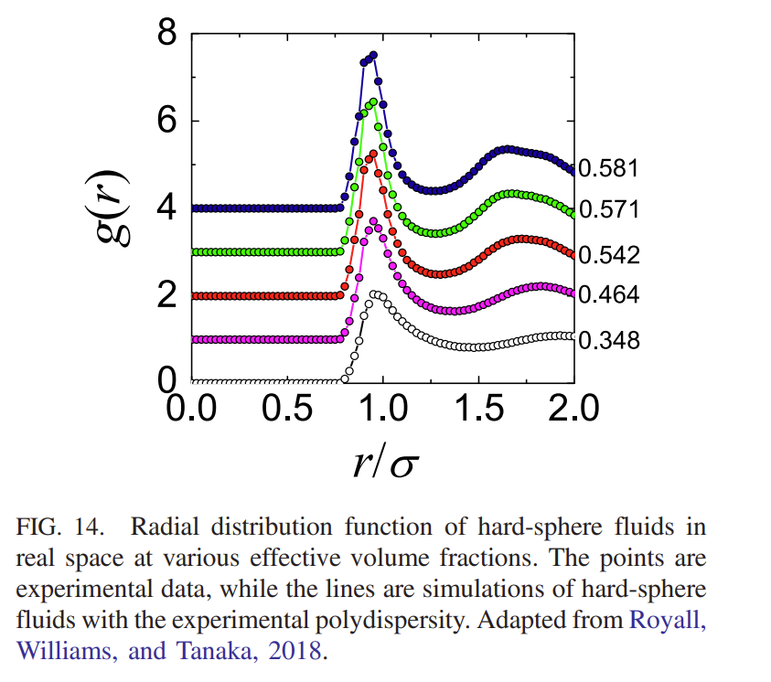
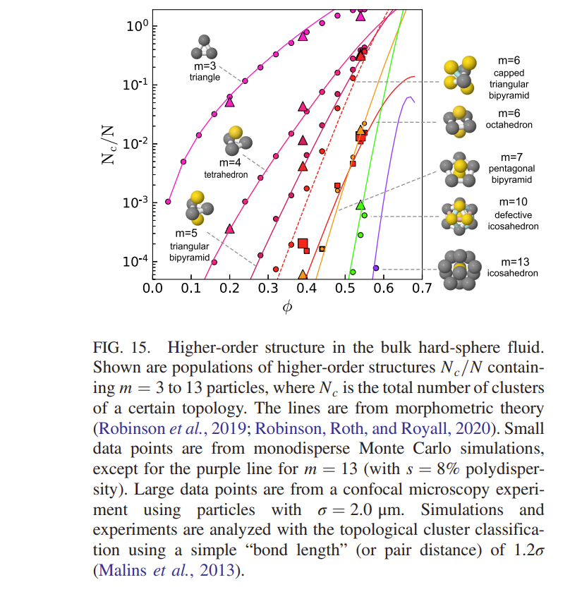
As mentioned previously, the early attempts at understanding the packing of particles in disordered materials came to te conclusion that 5 fold coordination (inconsistent with the long range order required for crystals) was the characteristic of simple dense packed structures. In the same spirit as these early experiments the results from confocal imaging have allowed the prevalence of different types of local ordering to be investigated. This leads to the mapping out the \(\textit{topological cluster distribution}\) (i.e. the different types of local structure) that occur in the system. As noted before, these higher order correlations may be calculated from the particle positions (once we have them) but cannot be determined unambiguously from measurements of \(g(r)\) alone.
These are just a few examples of the areas studied using colloids and confocal microscopy techqniues.
12.7 Calculation of \(g(r)\) directly from simulation
Although simulation is not strictly an experimental method, it is neither a truly theoretical method either. This said, from the experimentalist point of view, especially in the case of the colloind systems studied above, they provide a direct comparison in real space with the data. As such the experiemntal results are an important check of the veracity of the simulation methods especially with regard to the application of for example theoretical potentials. The simulation methods naturally exploit the interaction of the particles in real space (we know the positions of the particles and we calculate how they move under the influence of the interparticle forces. Hence, it is quite straight forward to compare the real space configurations measured in experiment with the particle coordinates in the simulation. The comparison between the experiment and simulation and the level of agreement that can be achieved can be strikingly seen in the comparison of \(g(r)\) for hard spheres shown above. Simulations however are not the answer to everything. They get more and more computer intensive as larger numbers of particles are included and the time scales over which they are carried out are extremely short compared to those in experiments. The latter is a particular issue with studies of the glass transition (as always) where the physical processes taking place may occur over a very wide range of timescales.
The comparison of simulation results with experimental diffraction data is more difficult. Diffraction experiments are a reciprocal space measurement and to compare to simulation we need to work out the corresponding real space (\(g(r)\) ) distributions. Hence when comparing experiment with simulation we have to choose whether to transform our reciprocal space data to real space (with associated problems) or convert the real space data from our simulations to reciprocal space for comparison (that also has problems). This is the subject of the next part of this course.
12.8 Dynamics in real space
Confocal microscopy experiments are not only useful for static measurements of \(g(r)\) but also open up the possibility for studying the dynamics of the system (how the particles move over time), that is, measurement of the time dependent pair correlation function \(G(r,t)\) I’ll not say much about dynamics at the present time but will leave it to the last part of this section of the course. Needless to say the process involves taking confocal images of the particles over time scales in which they will move only slightly from their initial position. With sophisticated software it is then possible to label the particles and track their position and hence coordinates in succesive image frames. This work well if you are in the sweet spot for the measurements but is a challenge, for example in glass transition experiments, where the experimental timescales become longer and longer as you approach the conditions for the glass transition to take place. This is still a very active field.
12.9 Summary and keypoints
In this section we have considered the experimental determination of \(g(r)\).
- We have seen that this is not realistically possible for atmonic systems,
- we have seen how colloid systems are ideal systems for studying the properties of hard-sphere and closely related systems on the 100nm scale,
- we have seen how \(g(r)\) for colloids may be obtained from the coordinates obtained from confocal microscopy,
- we have seen how \(g(r)\) and higher order correlations may be obtained from these coordinates,
- we have seen how we can extend the confocal microscopy method to study particle dynamics.