The concept of a random walk and its continuum limit – diffusion – introduced in the previous chapter, expresses the time evolution of the probability distribution \(p(x, t)\) for a particle’s position \(x\) by the diffusion equation:
\[
\frac{\partial p}{\partial t} = D \frac{\partial^2 p}{\partial x^2},
\]
which is a standard example of a so called Fokker-Planck equation, which is second-order in space and first-order in time.
In contrast, the Langevin equation provides a stochastic differential equation for the particle’s trajectory \(x(t)\). To understand it, consider the random hopping motion of a particle on a 1d lattice over a small time increment \(\Delta t\):
\[
x(t + \Delta t) = x(t) + \Delta x(t)
\]
Here, \(\Delta x(t)\) is a random displacement. If the lattice spacing is \(a\), we define the step statistics as:
\[
\Delta x(t) =
\begin{cases}
+a & \text{with probability } \nu \Delta t \\
-a & \text{with probability } \nu \Delta t \\
0 & \text{with probability } 1 - 2\nu \Delta t
\end{cases}
\]
This defines a discrete-time, discrete-space random walk. The average and variance of the step are easily derived (try as an exercise):
The mean displacement is \[
\langle \Delta x \rangle = (+a)(\nu \Delta t) + (-a)(\nu \Delta t) + 0(1 - 2\nu \Delta t) = 0.
\]
The mean square displacement is \[
\langle (\Delta x)^2 \rangle = (+a)^2(\nu \Delta t) + (-a)^2(\nu \Delta t) + 0^2(1 - 2\nu \Delta t)
= 2a^2\nu \Delta t.
\]
Hence the variance is \[
\mathrm{Var}(\Delta x) = \langle (\Delta x)^2 \rangle - \langle \Delta x \rangle^2 = 2a^2\nu \Delta t.
\]
Identifying \(D = a^2\nu\), we obtain \[
\langle (\Delta x)^2 \rangle = 2D\Delta t.
\]
The steps \(\Delta x(t)\) are uncorrelated across time.
To take the continuum limit, we let both \(a \to 0\) and \(\Delta t \to 0\), while keeping the diffusion constant \[
D = \nu a^2
\] fixed. This requirement implies that we need \(\nu\propto a^{-2}\), which is satisfied if \[
a \propto \sqrt{\Delta t}.
\]
Hence the step size must shrink as the square root of the time step. Only under this scaling does the random walk converge to a well-defined continuum process with finite diffusion constant, namely Brownian motion or the Langevin equation.
In this limit, we obtain the Langevin equation:
\[
\dot{x}(t) = \eta(t)
\]
where \(\eta(t)\equiv\frac{\Delta x(t)}{\Delta t}\) is a stochastic noise satisfying:
Comparing this with the diffusion equation result, we identify:
\[
\Gamma = 2D
\]
Hence, the Langevin description yields the same physical behavior — not just the mean-square displacement but also the full probability distribution \(p(x, t)\) — as the diffusion (Fokker-Planck) equation. This equivalence arises from the fact that the integral of many small, independent random steps leads to a Gaussian distribution, in agreement with the solution of the diffusion equation.
For more details, see: Stochastic Processes in Physics and Chemistry by N.G. van Kampen (North Holland, 1981).
9.2 Brownian Motion
Let us now examine Brownian motion, originally observed as the erratic motion of colloidal particles suspended in a fluid. These particles undergo constant collisions with surrounding (smaller) fluid molecules, which results in seemingly random movement.
From a coarse-grained perspective — where we do not track each individual collision — this appears as motion under random forces. This statistical treatment introduces irreversibility at the macroscopic level, even though the underlying molecular dynamics are reversible.
The Langevin equation provides a way to model this behavior. For a particle of mass \(m\) in one dimension, Langevin proposed the equation:
\[
m \ddot{x} = -\gamma \dot{x} + f(t)
\]
Here:
\(-\gamma \dot{x}\) is a frictional damping force, where \(\gamma\) is the damping coefficient.
\(f(t)\) is a random force due to molecular collisions.
Often, the mobility is defined as \(\mu = 1/\gamma\) — note that this is unrelated to chemical potential.
9.2.1 Noise Properties
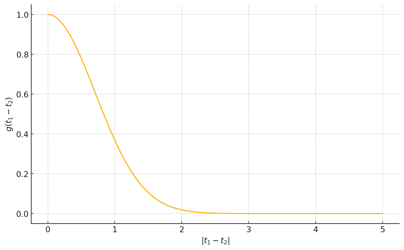
In principle the random forces are correlated in time since the molecular collisions which cause them are correlated and have some definite duration.
Let us assume that there is some correlation time \(t_c\) over which \(\langle f(t_1) f(t_2) \rangle = g(t_1 - t_2)\) decays rapidly as shown in the sketch below:
Figure 9.1: Sketch of \(g(t_1−t_2)\) against \(|t_1− t_2|\)
Then as long as we consider timescales \(\gg t_c\) we can safely replace \(g(t_1 - t_2)\) by a delta function. Thus we can make the approximation of white noise
We now averaging over all possible realisations of the random force, i.e we imagine repeating the Brownian motion experiment infinitely many times, each with a different random sequence of microscopic kicks \(f(t)\). Then
\[
\langle v(t) \rangle = v_0 e^{-\gamma t}
\] where we have used the fact that \(f(t)\) is random with \(\langle f(t)\rangle=0\). Thus:
At short times: (\(\gamma t \ll 1\)): \(\langle v \rangle \approx v_0\) ie. friction is negligible.
At long times: (\(\gamma t \gg 1\)): \(\langle v \rangle \to 0\) ie. the system loses memory of the initial velocity.
Adding both contributions: \[
\boxed{\langle [x(t) - x_0]^2 \rangle \approx v_0^2 t^2,}
\] which corresponds to ballistic motion (distance travelled is proportional to time).
Neglecting constant terms at large \(t\) gives: \[
\boxed{\langle [x(t) - x_0]^2 \rangle \simeq \frac{2k_B T}{\gamma}\, t,}
\] which corresponds to (distance travelled is proportional to \(\sqrt{t}\)) with diffusion constant \(D = \tfrac{k_B T}{\gamma}\).
The effective diffusion constant is:
\[
D = \frac{k_B T}{\gamma}
\]
This is the Einstein relation, connecting the rate of diffusion to temperature and damping. It is useful as it allows an explicit expression for the diffusion constant if one knows \(\gamma\). A famous example is a sphere: the equation for fluid flow past a moving sphere may be solved and yields \(\gamma=6\pi\eta a\) where \(a\) is the radius of the sphere and here \(\eta\) is the fluid viscosity. This gives
\[
D=\frac{k_BT}{6\pi\eta a}
\] which is the Stokes-Einstein formula for the diffusion constant of a colloidal particle.
9.2.5 External Forces and Mobility
Now consider a charged particle with charge \(q\) under an external electric field \(E\). The Langevin equation becomes:
\[
m \dot{v} = -\gamma v + qE
\]
At long times, the particle reaches a steady drift velocity:
\[
\langle v \rangle = \frac{qE}{\gamma} = \frac{qED}{k_B T}
\]
Defining the mobility \(\mu\) by \(\langle v \rangle = \mu qE\), we get the Nernst-Einstein relation:
\[
\mu = \frac{D}{k_B T}
\]
This relation connects the response of a system to an external perturbation (mobility) with its internal fluctuations (diffusivity).
9.2.6 Molecular Dynamics simulation of Brownian motion for a colloid particle in a liquid suspension