2 Key concepts for phase transitions
2.1 Observables and expectation values
In seeking to describe phase transition and critical phenomena, it is useful to have a quantitative measure of the difference between the phases: this is the role of the order parameter, \(Q\). In the case of the fluid, the order parameter is taken as the difference between the densities of the liquid and vapour phases. In the ferromagnet it is taken as the magnetisation. As its name suggest, the order parameter serves as a measure of the kind of orderliness that sets in when the temperature is cooled below a critical temperature.
Our first task is to give some feeling for the principles which underlie the ordering process. Referring back to Section 1.2, the probability \(p_a\) that a physical system at temperature \(T\) will have a particular microscopic arrangement (alternatively referred to as a ‘configuration’ or ‘state’), labelled \(a\), of energy \(E_a\) is
\[ p_a=\frac{1}{Z}e^{-E_a/k_BT} \tag{2.1}\]
The prefactor \(Z^{-1}\) is the partition function: since the system must always have some specific arrangement, the sum of the probabilities \(p_a\) must be unity, implying that
\[ Z=\sum_ae^{-E_a/k_BT} \tag{2.2}\] where the sum extends over all possible microscopic arrangements.
These equations assume that physical system evolves rapidly (on the timescale of typical observations) amongst all its allowed arrangements, sampling them with the probabilities Equation 2.1 the expectation value of any physical observable \(O\) will thus be given by averaging \(O\) over all the arrangements \(a\), weighting each contribution by the appropriate probability:
\[\overline {O}=\frac{1}{Z}\sum_a O_a e^{-E_a/k_BT} \tag{2.3}\]
Sums like Equation 2.3 are not easily evaluated because the number of terms grows exponentially in the system size. Nevertheless, some important insights follow painlessly. Consider the case where the observable of interest is the order parameter, or more specifically the magnetisation of a ferromagnet.
\[ Q=\frac{1}{Z}\sum_a Q_a e^{-E_a/k_BT} \tag{2.4}\]
It is clear from Equation 2.1 that at very low temperature the system will be overwhelmingly likely to be found in its minimum energy arrangements (ground states). For the ferromagnet, these are the fully ordered spin arrangements having magnetisation \(+1\), or \(-1\).
Now consider the high temperature limit. The enhanced weight that the fully ordered arrangement carries in the sum of Equation 2.4 by virtue of its low energy, is now no longer sufficient to offset the fact that arrangements in which \(Q_a\) has some intermediate value, though each carry a smaller weight, are vastly greater in number. A little thought shows that the arrangements which have essentially zero magnetisation (equal populations of up and down spins) are by far the most numerous. At high temperature, these disordered arrangements dominate the sum in Equation 2.4 and the order parameter is zero.
The competition between energy-of-arrangements weighting (or simply ‘energy’) and the ‘number of arrangements’ weighting (or ‘entropy’) is then the key principle at work here. The distinctive feature of a system with a critical point is that, in the course of this competition, the system is forced to choose amongst a number of macroscopically different sets of microscopic arrangements.
Finally in this section, we note that the probabilistic (statistical mechanics) approach to thermal systems outlined above is completely compatible with classical thermodynamics. Specifically, the bridge between the two disciplines is provided by the following equation
\[ F=-k_BT \ln Z \tag{2.5}\]
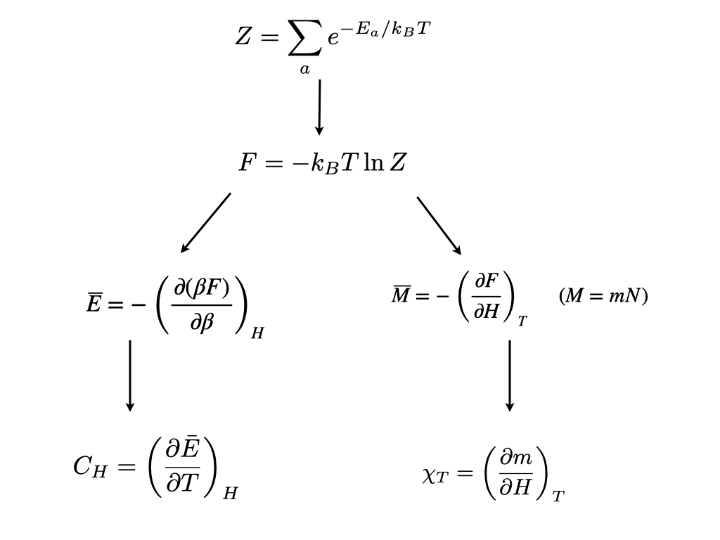
where \(F\) is the “Helmholtz free energy”. All thermodynamic observables, for example the order parameter \(Q\), and response functions such as the specific heat or magnetic susceptibility are obtainable as appropriate derivatives of the free energy. For instance, utilizing Equation 2.2, one can readily verify (try it as an exercise!) that the average internal energy is given by
\[\overline{E}=-\frac{\partial \ln Z}{\partial \beta},\]
where \(\beta=(k_BT)^{-1}\).
The relationship between other thermodynamic quantities and derivatives of the free energy are given in fig. Figure 2.1
2.2 Correlations
2.2.1 Spatial correlations
The two-point connected correlation function measures how fluctuations at two spatial points are statistically related. For a scalar field \(\phi(\vec{R})\), which could represent eg. the local magnetisation \(m\) in a magnet at position vector \(\vec{R}\), or the local particle number density \(\rho\) in a fluid, it is defined as:
\[ C(r) = \langle \phi(\vec{R}) \phi(\vec{R} + \vec{r}) \rangle - \langle \phi(\vec{R}) \rangle^2, \]
where \(\langle \cdot \rangle\) denotes an ensemble or spatial average over all \(\vec{R}\), and \(r = |\vec{r}|\) is the spatial separation between the two points.
\(C(r)\) quantifies the spatial extent over which field values are correlated and in homogeneous and isotropic systems, it depends only on the separation \(r\).
If \(C(r)\) decays quickly, we say that correlations are short-ranged. Typically this occurs well away from criticality and takes the form of exponential decay
\[ C(r) \sim e^{-r/\xi} \] where the correlation length \(\xi\) is the characteristic scale over which correlations decay.
Near a critical point \(C(r)\) decays more slowly - in a power-law fashion - and correlations are long-ranged.
\[ C(r) \sim r^{-(d - 2 + \eta)} \] where \(d\) is the spatial dimension and \(\eta\) is a critical exponent.
In isotropic fluids and particle systems, a closely related and more directly measurable quantity (particularly in simulations) is the radial distribution function \(g(r)\), which describes how particle density varies as a function of distance from a reference particle. For such systems, the two-point correlation function of the number density field \(\rho(\vec{r})\) is related to \(g(r)\) as follows:
\[ g(r) = 1+\frac{C(r)}{\rho^2}, \] where \(\rho\) is the average number density. This relation shows that \(g(r)\) encodes the same spatial correlations as \(C(r)\), but in a form that is more natural for discrete particle systems. Note that by definition \(g(r)\to 1\) in the absence of correlations ie. when \(C(r)=0\). This is typically the case for \(r\gg\xi\).
Experimentally one doesn’t typically have direct access to \(C(r)\), but rather its Fourier transform known as the structure factor
\[ S(k) = \int d^d r \, e^{-i \vec{k} \cdot \vec{r}} \, C(r), \] where \(k\) is the scattering wavevector and \(d^dr\) refers to the elemental volume (eg. \(d^3r\) in three dimensions).
In equilibrium:
For short-range correlations (finite \(\xi\)), \(S(k)\) typically has a Lorentzian form: \[ S(k) \sim \frac{1}{k^2 + \xi^{-2}}. \]
At criticality (where \(\xi \to \infty\)), \(S(k)\) follows a power law: \[ S(k) \sim k^{-2 + \eta}. \]
This relation enables the extraction of \(\xi\) from experimental or simulation data, especially via scattering techniques.
2.2.2 Temporal correlations
Consider a thermodynamic variable \(x\) with zero mean that fluctuates over time. Examples include the local magnetization in a magnetic system or the local density in a fluid. Here, \(x\) represents a deviation from the average value — a fluctuation.
We’re interested in how such fluctuations are correlated over time when the system is in thermal equilibrium. For instance, if \(x\) is positive at some time \(t\), it’s more likely to remain positive shortly after.
These temporal correlations are characterized by the two-time correlation function (also known as an auto-correlation function):
\[ \langle x(\tau) x(\tau + t) \rangle \]
In equilibrium, the correlation function must be independent of the starting time \(\tau\). Therefore, we define:
\[ \langle x(\tau) x(\tau + t) \rangle = M_{xx}(t) \]
That is, \(M_{xx}(t)\) depends only on the time difference \(t\).
We typically expect \(M_{xx}(t)\) to decay exponentially over a characteristic correlation time \(t_c\):
\[ M_{xx}(t) \sim \exp(-t / t_c) \]
.png)
This exponential decay reflects how the memory of fluctuations fades with time.
Now consider two different fluctuating variables, \(x\) and \(y\) (e.g., local magnetizations at different positions). Their cross-correlation function is defined as:
\[ \langle x(\tau) y(\tau + t) \rangle = M_{xy}(t) \]
This defines the elements of a dynamic correlation matrix, of which \(M_{xx}(t)\) is the diagonal.