6 The Static Scaling Hypothesis
Historically, the first step towards properly elucidating near-critical behaviour was taken with the static scaling hypothesis. This is essentially a plausible conjecture concerning the origin of power law behaviour which appears to be consistent with observed phenomena. According to the hypothesis, the basis for power law behaviour (and associated scale invariance or “scaling”) in near-critical systems is expressed in the claim that: in the neighbourhood of a critical point, the basic thermodynamic functions (most notably the free energy) are generalized homogeneous functions of their variables. For such functions one can always deduce a scaling law such that by an appropriate change of scale, the dependence on two variables (e.g. the temperature and applied field) can be reduced to dependence on one new variable. This claim may be warranted by the following general argument.
A function of two variables \(g(u,v)\) is called a generalized homogeneous function if it has the property
\[g(\lambda^au,\lambda^bv)=\lambda g(u,v)\] for all \(\lambda\), where the parameters \(a\) and \(b\) (known as scaling parameters) are constants. An example of such a function is \(g(u,v)=u^3+v^2\) with \(a=1/3, b=1/2\).
Now, the arbitrary scale factor \(\lambda\) can be redefined without loss of generality as \(\lambda^a=u^{-1}\) giving
\[g(u,v)=u^{1/a}g(1,\frac{v}{u^{b/a}})\] A corresponding relation is obtained by choosing the rescaling to be \(\lambda^b=v^{-1}\).
\[\label{eq:sca2} g(u,v)=v^{1/b}g(\frac{u}{v^{a/b}},1)\]
This equation demonstrates that \(g(u,v)\) indeed satisfies a simple power law in \(\mathit{one}\) variable, subject to the constraint that \(u/v^{a/b}\) is a constant. It should be stressed, however, that such a scaling relation specifies neither the function \(g\) nor the parameters \(a\) and \(b\).
Now, the static scaling hypothesis asserts that in the critical region, the free energy \(F\) is a generalized homogeneous function of the (reduced) thermodynamic fields \(t=(T-T_c)/T_c\) and \(h=(H-H_c)\). Remaining with the example ferromagnet, the following scaling assumption can then be made:
\[F(\lambda^a t,\lambda^b h)=\lambda F(t,h) \:. \label{eq:scagibbs}\]
Without loss of generality, we can set \(\lambda^a=t^{-1}\), implying \(\lambda=t^{-1/a}\) and \(\lambda^b=t^{-b/a}\).
Then \[F(t,h)=t^{1/a}F(1,t^{-b/a}h)\] where our choice of \(\lambda\) ensures that \(F\) on the rhs is now a function of a single variable \(t^{-b/a}h\).
Now, as stated in Chapter 2, the free energy provides the route to all thermodynamic functions of interest. An expression for the magnetisation can be obtained simply by taking the field derivative of \(F\) (cf. Figure 2.1)
\[m(t,h)=(-t)^{(1-b)/a}m(1,t^{-b/a}h) \tag{6.1}\]
In zero applied field \(h=0\), this reduces to
\[m(t,0)=(-t)^{(1-b)/a}m(1,0)\] where the r.h.s. is a power law in \(t\). Equation 3.4 then allows identification of the exponent \(\beta\) in terms of the scaling parameters \(a\) and \(b\).
\[\beta=\frac{1-b}{a}\]
By taking further appropriate derivatives of the free energy, other relations between scaling parameters and critical exponents may be deduced. Such calculations (Exercise: try to derive them) yield the results \(\delta = b/(1-b)\),\(\gamma = (2b-1)/a\), and \(\alpha =(2a-1)/a\) . Relationships between the critical exponents themselves can be obtained trivially by eliminating the scaling parameters from these equations. The principal results (known as “scaling laws”) are:- \[ \begin{aligned} \alpha+\beta(\delta+1)=2 \\ \alpha+2\beta+\gamma=2 \end{aligned} \]
Thus, provided all critical exponents can be expressed in terms of the scaling parameters \(a\) and \(b\), then only two critical exponents need be specified, for all others to be deduced. Of course these scaling laws are also expected to hold for the appropriate thermodynamic functions of analogous systems such as the liquid-gas critical point.
6.1 Experimental Verification of Scaling
The validity of the scaling hypothesis finds startling verification in experiment. To facilitate contact with experimental data for real systems, consider again Equation 6.1. Eliminating the scaling parameters \(a\) and \(b\) in favour of the exponents \(\beta\) and \(\delta\) gives
\[ \frac{m(t,h)}{t^{\beta}}=m(1,\frac{h}{t^{\beta\delta}}) \] where the RHS of this last equation can be regarded as a function of the single scaled variable \(\tilde{H} \equiv t^{-\beta\delta} h(t,M)\).
For some particular magnetic system, one can perform an experiment in which one measures \(m\) vs \(h\) for various fixed temperatures. This allows one to draw a set of isotherms, i.e. \(m-h\) curves of constant \(t\). These can be used to demonstrate scaling by plotting the data against the scaling variables \(M=t^{-\beta}m(t,h)\) and \(\tilde{H}=t^{-\beta\delta}h(t,M)\). Under this scale transformation, it is found that all isotherms (for \(t\) close to zero) coincide to within experimental error. Reassuringly, similar results are found using the scaled equation of state of simple fluid systems such as He\(^3\) or Xe.

In summary, the static scaling hypothesis is remarkably successful in providing a foundation for the observation of power laws and scaling phenomena. However, it furnishes little or no guidance regarding the role of co-operative phenomena at the critical point. In particular it provides no means for calculating the values of the critical exponents appropriate to given model systems.
6.2 Computer simulation
In seeking to employ simulation to obtain estimates of bulk critical point properties (such as the location of a critical point and the values of its associated exponents), one is immediately confronted with a difficulty. The problem is that simulations are necessarily restricted to dealing with systems of finite-size and cannot therefore accommodate the truly long ranged fluctuations that characterize the near-critical regime. As a consequence, the critical singularities in \(C_v\), order parameter, etc. appear rounded and shifted in a simulation study. Figure 6.2 shows a schematic example for the susceptibility of a magnet.
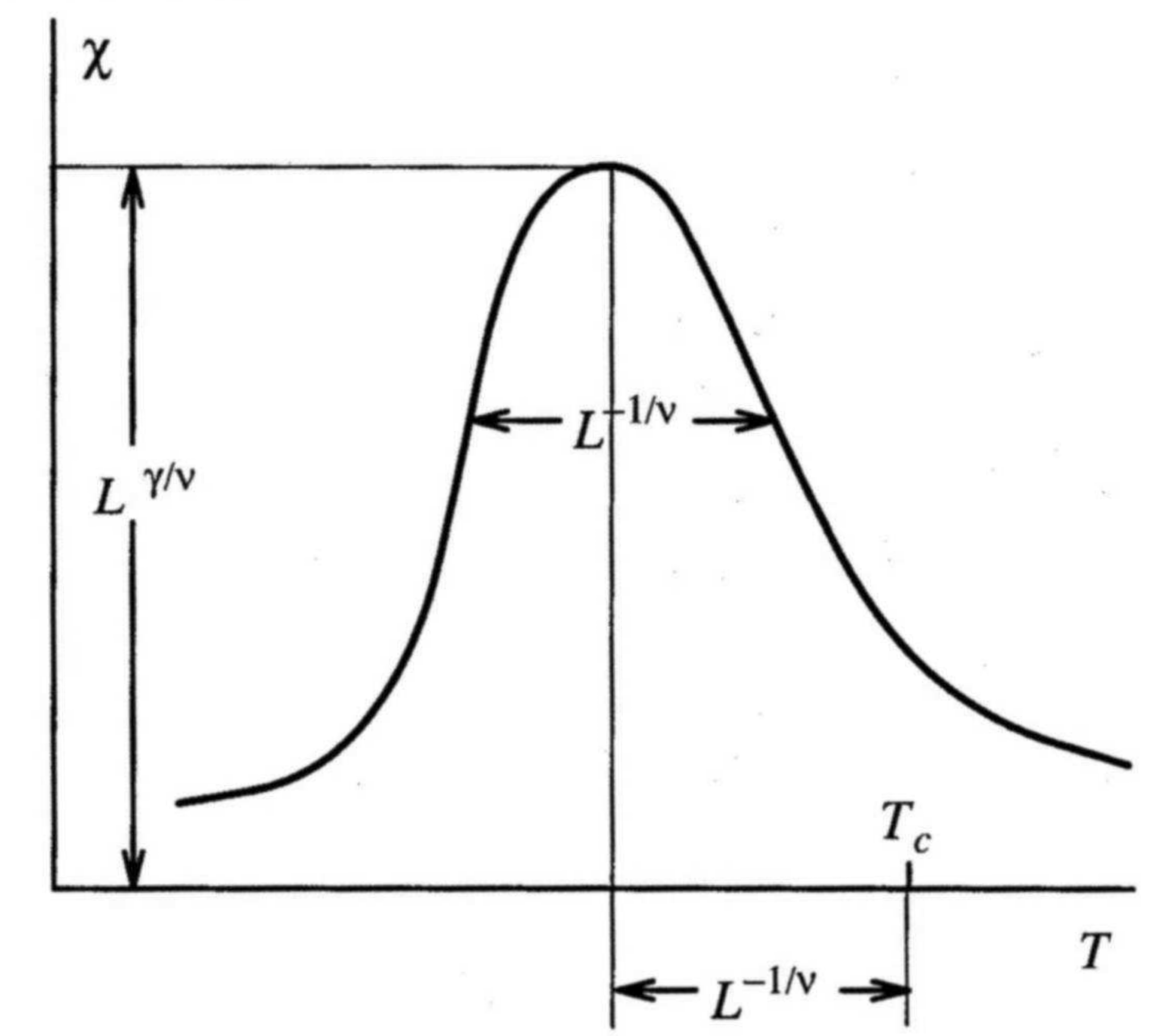
Thus the position of the peak in a response function (such as \(C_v\)) measured for a finite-sized system does not provide an accurate estimate of the critical temperature. Although the degree of rounding and shifting reduces with system size, it is often the case, that computational constraints prevent access to the largest system sizes which would provide accurate estimates of critical parameters. To help deal with this difficulty, finite-size scaling (FSS) methods have been developed to allow extraction of bulk critical properties from simulations of finite size. FSS will be discussed in section 7.