20  Measurements in reciprocal space

20.1 Diffraction

In the previous experimental section we saw how measurements of \(g(r)\) may be made by directly finding coordinates of particles in space. We saw how this could be applied to colloidal systems. The optical methods applied are confined to systems at or close to the diffraction limit, that for optical wavelengths is a few hundred nanometres. Another problem that may arise is that \(g(r)\) is a statistical quantity and to obtain meaningful results it must be calculated over a large number of particle positions and care must be taken to ensure that the system under study is homogeneous.

In order to determine \(g(r)\) directly in a similar way for atomic and molecular systems we would need to use wavelengths that are much less than the atomic size, that is beyond X-ray wavelengths. This is not practical. In contrast, it is possible to image at the atomic scale using electron microscopy. However, in this case it is not possible to image in the bulk in a similar way to confocal microscopy and studies are largely limited to 2D surfaces. Hence, most studies at this scale are based on diffraction methods - the topic of this part of the course.

Optically, you are aware from your study of waves that diffraction effects occur when the scale of the structure is of the same order of the wavelength of light. The same principle applies for atomic scales which means diffraction needs wavelengths around 0.1 nanometres (or 1 Å) for atomic scale studies.

0.1 nm is in the X-ray regime but it’s also accessible with thermal neutrons (~ 300K is approximately 0.18 nm) or electrons. (Exercise. Calculate the energy of a photon, neutron and electron corresponding to a wavelength of 0.1 nm.).

So how do we use diffraction in disordered systems to obtain structural information such as \(g(r)\)?

20.2 The structure factor - a simple approach.

We will not use a rigorous approach to diffraction (that requires quantum mechanics) but we will approach the relationship between the scattering of x-rays, neutrons and electrons by atoms by considering the following simple picture. We note that we haven’t included the strength or the specific way in which the atoms scatter at this point but have assumed an incoming quantum is scattered by the atoms. We also assume for the moment that we only have one atom type.

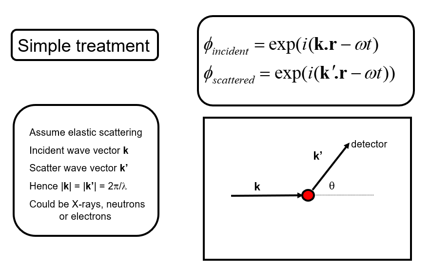
We then wish to understand how the scattered waves from different atoms interfere to give rise to a diffraction pattern (for example scattered intensity vs. angle).

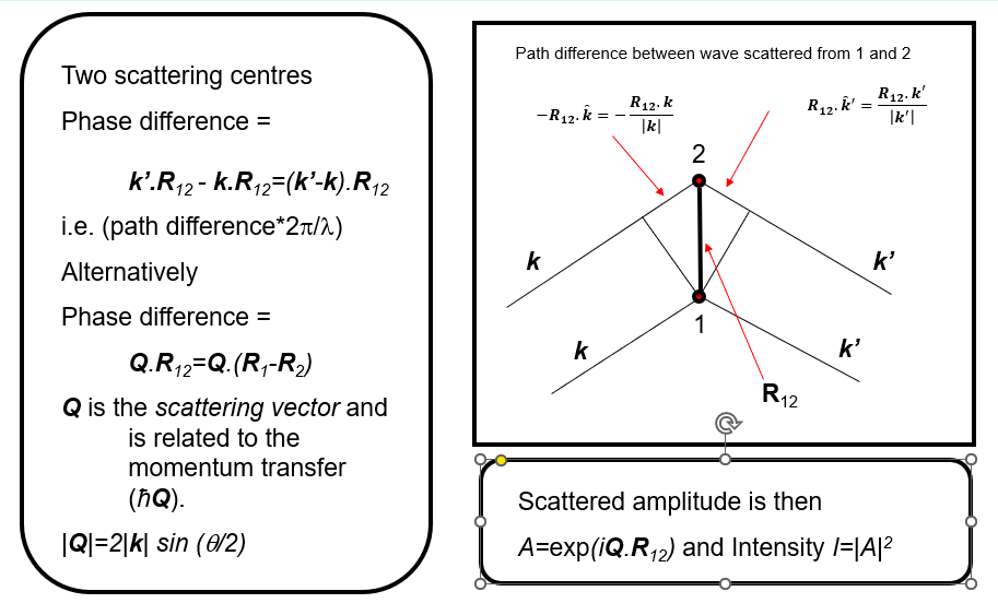
We can write the structure factor (beware, if you are familiar with crystal diffraction, this is a different definition for the structure factor) for the scattering of all the atoms in the material as

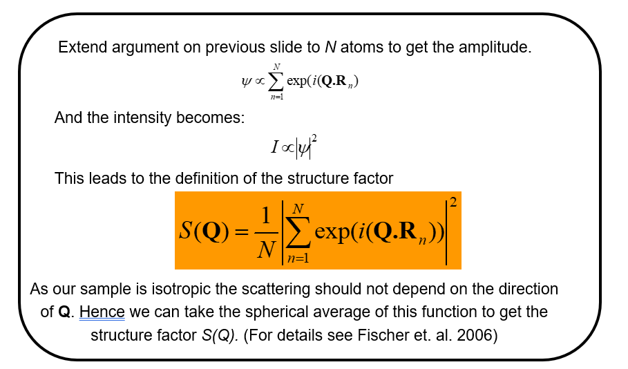
We note that \(N\) is just a normalizing factor to give the scattering per atom and that for a liquid we need to take the spherical average of this function to return a function \(S(Q)\) that is isotropic (the same in all directions). (NB. This latter step would not be taken, in for example representing the scattering from a liquid crystal, where we know there is an orientation of the molecules in the liquid - the director - even though there is still liquid like disorder in the other directions).

A more formal derivation of the structure factor obtained in a scattering experiment for a single element may be found in Fischer et al. 2006 and may be written in terms of the differential scattering cross-section,

\[\frac{1}{N} \frac{d\sigma}{d\Omega}=b^2_{coh}S(Q)+b^2_{incoh}\]

for neutrons where \(b_{coh}\) is the coherent scattering length of the element and \(b_{incoh}\) is the incoherent scattering length that arises due to the difference in scattering by the nucleus when its nuclear spin (if it has a spin) is aligned or anti-aligned with the neutron and/or when it is different due to the nuclear scattering arising from different isotopes of the same element.

For the case of X-rays the corresponding quantity, in its simplest form is,

\[\frac{1}{N} \frac{d\sigma}{d\Omega}=f(Q)^2 S(Q)\]

where we note this is after corrections for the effects of polarization of the x-ray beam in the incident and scattered beam has been made.

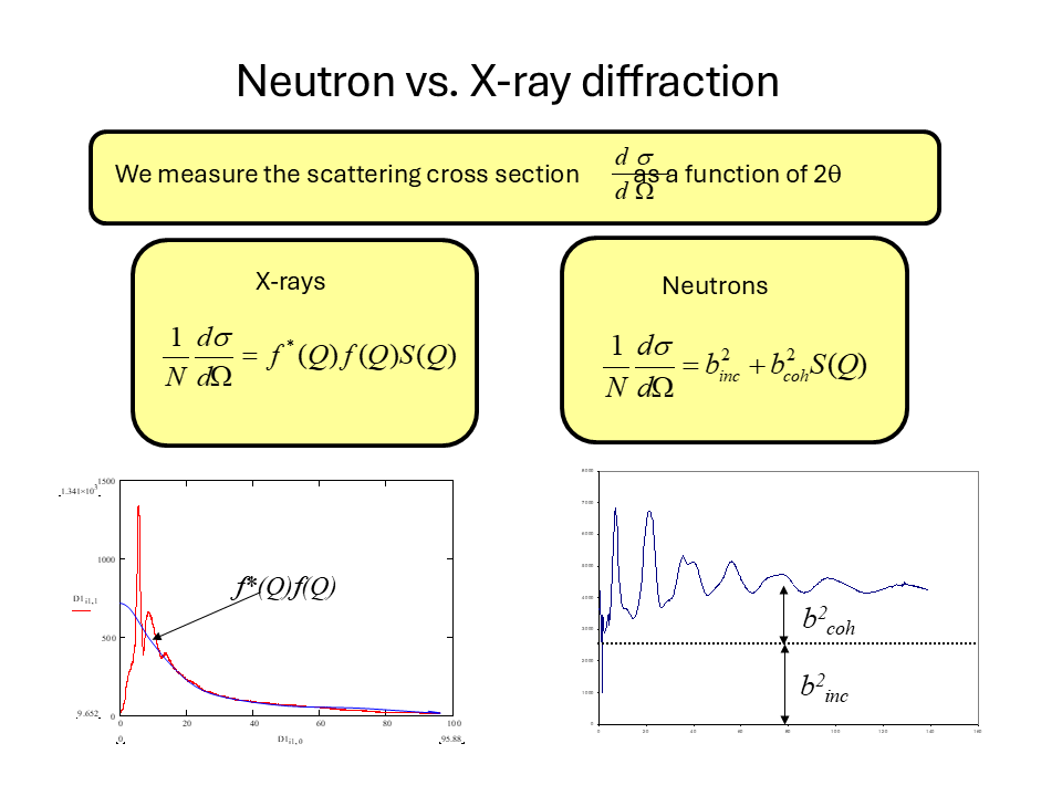
From the figure we note the important difference between the neutron and X-ray diffraction patterns. At large values of \(Q\) the neutron diffraction cross-section tends to a constant value \(b^2_{coh}+b^2_{incoh}\) whereas for X-rays we see that the diffraction tends to zero at large \(Q\) due to the \(Q\) dependence of the X-ray form factor. The physical origin of this effect is that for neutrons it is the nucleus (with a size of a few femtometres) that is the scattering object whereas for X-rays it is the electron cloud around the atom (with dimensions of about a tenth of a nanometer) that is the scattering object. Hence for a thermal neutron (of wavelength 0.18 nm) the atoms in the material act as point scatterers whereas the scattering from X-rays is for an object of roughly the same wavelength. Hence the shape of \(f(Q)\) reflects the distribution of the electrons around the atom. This \(Q\) dependence of the form factor has important consequences when we consider materials composed of more than one element as we shall see shortly.

[The effect is equivalent in optics to the difference from the diffraction pattern from a grating that is composed of very narrow slits compared to one composed of slit widths on the same scale as their separation cf.

\[I\sim \left(\frac{\sin \alpha}{\alpha}\right)^2\left(\frac{\sin N\beta}{\sin\beta}\right)^2\]]

We also note that both \(b\) and \(f(Q)\) should be considered as complex quantities (that give rise to absorption and alter the scattering cross-section close to a neutron resonance or X-ray absorption edge).

Hence, provided we are able to make the experimental corrections we can see that, at least for a single element, \(S(Q)\) for the liquid or glass may be obtained directly.

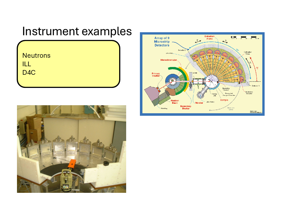
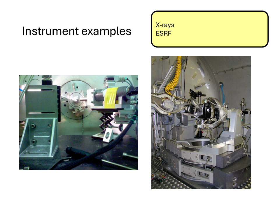
Here are some images of some typical X-ray and neutron diffractometers at the ILL and ESRF central facilities.

20.3 The relationship between \(S(Q)\) and \(g(r)\) for a disordered material.

The description above gives insight into the origins of the interference (diffraction) effects observed from a disordered arrangement of scatterers. There is a direct sine Fourier transform pair relationship between the radial distribution function \(g(r)\) and the structure factor \(S(Q)\) for the material and is as follows.

\[S(Q)=1+\frac{4\pi\rho}{Q}\int_0^{\infty}r(g(r)-1)\sin(Qr)dr\]

and

\[g(r)=1+\frac{1}{2\pi\rho r}\int_0^{\infty}Q(S(Q)-1)\sin(Qr)dQ\]

Again, we note that these quantities do not depend on the nature of the scattering. Hence, by measuring \(S(Q)\) we can in principle obtain \(g(r)\).

20.4 Practical points

In practice it is not possible to measure the complete \(S(Q)\) function in an experiment. Apart from statistical and systematic uncertainties in the measurements, we see the maximum value of \(Q\) that can be measured is determined by the maximum scattering angle and the wavelength of the x-ray, neutron etc. So for \(2\theta= 180^\circ\) (\(\pi\)), the maximum possible scattering angle, we obtain \(Q_{\max}=\frac{4\pi}{\lambda}\), where \(\lambda\) is the wavelength. We will also find there is a minimum value of \(Q\), \(Q_{\min}\) that is determined by the divergence of the incident beam and the distance and shielding of the detector. Hence in the transform from \(S(Q)\) to \(g(r)\) the limits are \(Q_{\min}\) and \(Q_{\max}\) that are determined by experimental constraints.

\(Q_{\min}\) sets the limit on the extent of the long-range structure that we may observe. For example, correlations at long length scales could give rise to peaks that occur below \(Q_{\min}\) and hence be unobservable. So, if the aim of your study is to look at long-range correlations (i.e. between large molecules for example) you aim to get as low in \(Q\) as possible. This is usually achieved by using longer wavelength X-rays or neutrons. For example, for neutron scattering, experiments to observe small \(Q\) scattering (sometimes misleadingly termed small angle scattering) instruments use neutrons from a ‘cold source’ of neutrons (typically from a moderator using liquid deuterium (25K or ~ 4Å) at the ILL or liquid methane (50K) at ISIS. For X-rays you would select sources and instruments optimised for X-ray wavelengths below 10 keV.

\(Q_{\max}\) determines the amount of detail you can see at shorter ranges. If it is not high enough you won’t be able to resolve anything on the atomic length scales. A general rule of thumb for disordered materials is you need to measure to the point where there appears to be no structure in the diffraction pattern at the highest \(Q\) values. Hence X-ray and neutron diffractometers for studying atomic materials and in particularly glasses use short wavelength neutrons or X-rays. For neutrons, the neutrons are obtained from a ‘hot source’ moderator (the graphite moderator at the ILL works at 3000K and has the maximum flux at about 0.5 Å) or the instruments are designed to exploit the high energy epi-thermal neutrons from a pulse source (i.e. ISIS). The more locally ordered the material (for example an oxide glass versus a high temperature liquid) the higher in \(Q\) one needs to go. For the hot source instruments you typically get 23 Å\(^{-1}\). For pulsed neutron sources \(Q\) values of 50 Å\(^{-1}\) may be achieved.

At this point, hopefully, you should see the difficulty - optimising for \(Q_{\min}\) compromises your high \(Q_{\max}\) and vice versa for single wavelength instruments. Hence, you typically need to make a careful choice of instrument or instruments depending on the material to be studied.

The situation at ‘time of flight’ neutron sources (such as ISIS) is slightly different as it is possible to simultaneously obtain lower \(Q_{\min}\) and higher \(Q_{\max}\) than using a single wavelength diffractometer. We don’t have time to go into details here but needless to say there are further experimental difficulties to consider when you go down that route.

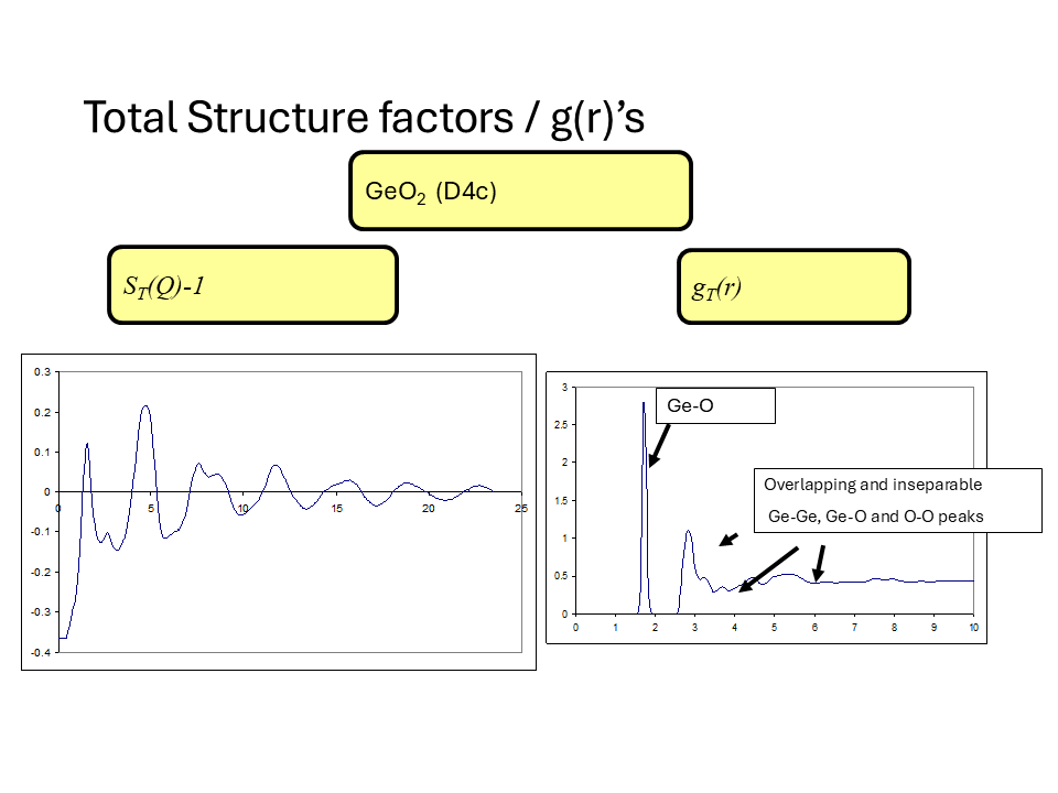
20.5 Partial Structure Factors

As we noted previously, the discussion so far has only considered mono-atomic systems - a very limited case! In reality we deal with materials that contain more than one atom type and hence we need a way to describe the arrangements of different types of atom around each other. i.e. How do we interpret the diffraction pattern from a multicomponent system? Well, we can extend our idea of the radial distribution function and introduce the idea of a partial radial distribution function, \(g_{\alpha\beta}(r)\), which may be described as the radial distribution function for the arrangement of atoms of type \(\beta\) around those of type \(\alpha\). We note also that \(\alpha\) and \(\beta\) can represent the same atom type. Take for example a glass such as germanium dioxide (\(GeO_2\)). We can define four partial radial distribution functions, \(g_{GeGe}(r)\) describing the distribution of the germanium atoms around a germanium atom at the origin, \(g_{OO}(r)\) describing the distribution of oxygen atoms around an oxygen atom at the origin and \(g_{GeO}(r)\) describing the distribution of oxygen atoms around a germanium atom at the origin and vice versa (\(g_{OGe}(r)\)). With a little thought we can also see that \(g_{GeO}(r)=g_{OGe}(r)\) so that for our binary system we only need 3 partial radial distribution functions to describe the structure. Extending the arguments we used previously, we may then define the partial structure \(S_{\alpha\beta}(Q)\) as,

\[S_{\alpha\beta}(Q)=1+ \frac{4\pi\rho}{Q}\int_0^{\infty}r(g_{\alpha\beta}(r)-1)\sin(Qr)dr\]

for which the inverse transform is,

\[g_{\alpha\beta}(r)=1+\frac{1}{2\pi\rho r}\int_0^{\infty}Q(S_{\alpha\beta}(Q)-1)\sin(Qr)dQ\]

20.6 Diffraction from multicomponent systems.

We see each \(S_{\alpha\beta}(Q)\) that are related to the positions of the diffracting pairs above, will contribute to the diffraction pattern for our multicomponent system. We expect the contribution to the intensity from each \(S_{\alpha\beta}(Q)\) to depend on the strength of the scattering from the atom type involved (i.e. \(b_{coh}\) or \(f(Q)\)) and its concentration (\(c_\alpha\) and \(c_\beta\)). So, in the case of a multicomponent system we write our scattering cross-section (again after experimental corrections) as,

\[\frac{1}{N} \frac{d\sigma}{d\Omega}=\sum_{\alpha=1}^N\sum_{\beta=1}^Nc_{\alpha}c_{\beta}b_{coh,\alpha}b_{coh,\beta}S_{\alpha\beta}(Q)+\sum_{\alpha=1}^Nb^2_{\alpha,incoh}\]

for the case of neutron scattering.

This may be re-written as

\[\frac{1}{N} \frac{d\sigma}{d\Omega}=F^N(Q)+\sum_{\alpha=1}^N\sum_{\beta=1}^Nc_{\alpha}c_{\beta}b_{coh,\alpha}b_{coh,\beta}+\sum_{\alpha=1}^Nb^2_{\alpha,incoh}\]

where we have defined

\[F^N(Q)=\sum_{\alpha=1}^N\sum_{\beta=1}^Nc_{\alpha}c_{\beta}b_{coh,\alpha}b_{coh,\beta}(S_{\alpha\beta}(Q)-1)\]

For the case of X-ray scattering we have

\[\frac{1}{N} \frac{d\sigma}{d\Omega}=\sum_{\alpha=1}^N\sum_{\beta=1}^Nc_{\alpha}c_{\beta}f_{\alpha}(Q)f_{\beta}(Q)S_{\alpha\beta}(Q)\]

or

\[\frac{1}{N} \frac{d\sigma}{d\Omega}=F^X(Q)+\sum_{\alpha=1}^N\sum_{\beta=1}^Nc_{\alpha}c_{\beta}f_{\alpha}(Q)f_{\beta}(Q)\]

where,

\[F^X(Q)=\sum_{\alpha=1}^N\sum_{\beta=1}^Nc_{\alpha}c_{\beta}f_{\alpha}(Q)f_{\beta}(Q)(S_{\alpha\beta}(Q)-1)\]

Hence we see \(F^N(Q)\) and \(F^X(Q)\) contain all the structure information in the scattering but at the same time we see that the individual partial structure factors can not be isolated in a single diffraction pattern. The sine Fourier transform of \(F^N(Q)\) gives,

\[G^N(r)=\sum_{\alpha=1}^N\sum_{\beta=1}^Nc_{\alpha}c_{\beta}b_{coh,\alpha}b_{coh,\beta}+\frac{1}{2\pi\rho r}\int_0^{\infty}F^N(Q)\sin(Qr)dQ\]

or,

\[G^N(r)=\sum_{\alpha=1}^N\sum_{\beta=1}^Nc_{\alpha}c_{\beta}b_{coh,\alpha}b_{coh,\beta}+\sum_{\alpha=1}^N\sum_{\beta=1}^Nc_{\alpha}c_{\beta}b_{coh,\alpha}b_{coh,\beta}(g_{\alpha\beta}(r)-1)\]

where we’ve applied the sine Fourier transform of \(F^N(Q)\) to get the total radial distribution function that is just the weighted sum of the partial radial distribution functions. For X-rays the equivalent sine Fourier transform,

\[\frac{1}{2\pi\rho r}\int_0^{\infty}F^X(Q)\sin(Qr)dQ\]

is no longer a linear combination of the partial radial distribution functions as the \(Q\) dependence of the form factors acts as a ‘modification’ function on the transform that has the effect of broadening the peaks in real space. Also, as the \(Q\) dependence of the form factors is different for each element (related to the size of the atom) the effect of this broadening will be different for each \(g_{\alpha\beta}(r)\). In much experimental x-ray work this broadening effect is often reduced by dividing \(F^X(Q)\) by the weighted sum of the form factor terms. This has the effect of reducing the peak broadening at the expense of some distortion in the partial \(g(r)\)s.

20.7 Neutron diffraction and isotope substitution

We have seen that it is not possible, in a single neutron or X-ray diffraction experiment, to obtain the partial radial distribution functions of a disordered material. So in a simple measurement, the interpretation (e.g. assignment of bond distances, coordination numbers …) of \(G(r)\) is by assignment and fitting overlapping peaks. More recently, rather than fitting peaks, the trend is for data to be directly compared to the structures calculated from computer simulations (Monte Carlo or Molecular Dynamics) and/or by refining (by fitting) the simulation structures to obtain agreement with the experimental data. However, both methods inevitably limit the precision of the structure determination possible.

However, as we have seen, the neutron scattering cross-section depends on the properties of the nucleus of the atom, that is in itself dependent on the atomic weight, and not the atomic number of the element in question. In particular, \(b_{coh}\) depends on the isotope of the element. Hence, the scattering cross-section of a material will be different if its isotopic composition is changed. However, its chemical properties will remain unchanged. This difference in scattering from different isotopes is exploited in the technique of neutron diffraction and isotopic substitution (NDIS). Take for example our \(GeO_2\) glass. We can make this glass from Germanium with its natural abundance of elements or we can use isotopically enriched samples made with Ge\(^{70}\) and Ge\(^{73}\). The different coherent neutron scattering lengths for oxygen and these germanium isotopes are shown in the table below.

isotope	scattering length /fm
Ge (Natural)	8.185
Ge (70)	10.00
Ge (73)	5.02
O (Natural)	5.802

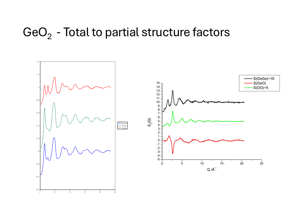
The concentrations of the germanium and oxygen atoms are \(c_{Ge}=1/2\) and \(c_O=2/3\) so the relative weightings of the three partial structure factors in \(F^N\) are different for the differently isotopically labelled samples so that the diffraction pattern observed will be different for each case. We can express the difference in matrix form

\[\begin{pmatrix} 0.074&0.150&0.211\\0.110&0.150&0.256\\0.030&0.150&0.133\end{pmatrix}\begin{pmatrix}S_{GeGe}(Q)\\S_{OO}(Q)\\S_{GeO}(Q)\end{pmatrix}=\begin{pmatrix}F^N_{nat}(Q)\\F^N_{70}(Q)\\F^N_{73}(Q)\end{pmatrix}\]

from which we can see that we have three measurements (the \(F^N(Q)\) for the different isotope compositions) and three unknowns (the partial \(S_{\alpha\beta}(Q)\)). Hence, we can determine \(S_{GeGe}(Q)\), \(S_{OO}(Q)\) and \(S_{GeO}(Q)\) by multiplying the left and right side of this equation by the inverse matrix to obtain,

\[\begin{pmatrix}S_{GeGe}(Q)\\S_{OO}(Q)\\S_{GeO}(Q)\end{pmatrix}=\begin{pmatrix} -171&108&63\\-65&34&38\\111&-62&-49\end{pmatrix}\begin{pmatrix}F^N_{nat}(Q)\\F^N_{70}(Q)\\F^N_{73}(Q)\end{pmatrix}\]

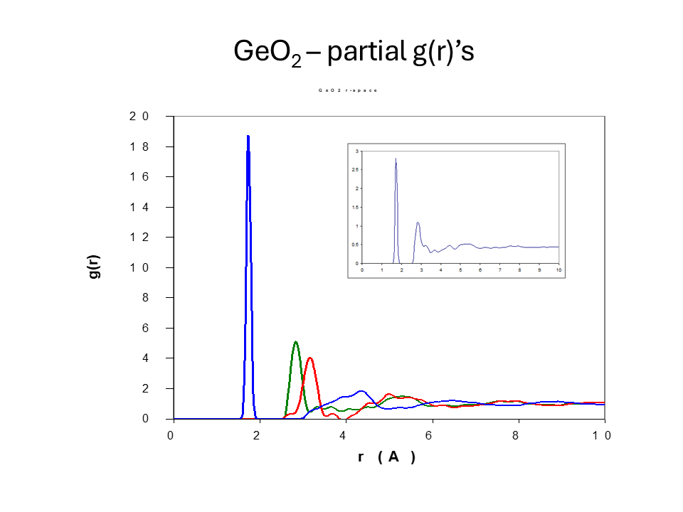
The figures below show the measured \(F^N(Q)\) for these isotopically labelled glasses and the partial structure factors obtained by this matrix inversion. The \(g_{\alpha\beta}(r)\) obtained by Fourier transform of the partial structure is shown below in addition to the total \(G(r)\) for the natural sample.

It is important to note some of the limitations of this method

• not all elements have isotopes or isotopes with large differences in scattering length,
• isotopically enriched elements are very expensive, tens of thousands of dollars per gram,
• even with good scattering length variation, the scattering matrix is still typically poorly conditioned (see the statistical errors on the data above),
• it is only realistic for binary systems, the scattering matrix for ternary (3x3) or higher compounds is poor even for the best isotopes available.

One variation that was demonstrated for \(GeO_2\) is to consider an X-ray diffraction measurement as one of the ‘isotopic’ compositions. In this case the inverse matrix will vary with \(Q\) due to the X-ray form factors, but the partial structure factors can still be formally calculated using the inverse matrix at each \(Q\) point.

20.8 Difference diffraction experiments

As noted above, the number of cases where formal inversion to partial structures may be obtained is very limited. However, difference or contrast techniques are much more commonly applied. In this case, a single isotopic change is made in the material. Inspection of the weightings then shows that a simple subtraction of one diffraction pattern from the other (provided they are properly corrected and normalised) removes all correlations apart from those that involve the substituted atom. In addition, by suitable weighting of one pattern it is possible to remove all the contributions from the substituted atom apart from \(S_{\alpha\alpha}(Q)\) (which is generally small anyway).

These difference techniques have been used extensively in the study of the hydration of ions in aqueous solutions and the coordination of metal ions in oxide glasses to name a few.

A related technique - X-ray anomalous (resonant) scattering - where variations in \(f(Q)\) has been exploited in a few cases.

20.9 Spectroscopy - EXAFS, XANES, NMR …

Diffraction experiments, especially when used with substitution techniques give structural information to large \(r\) in \(g(r)\). However, the techniques can be difficult and expensive to carry out. Hence spectroscopic techniques, that are usually very sensitive to local atomic configurations, are also used extensively in the study of disordered materials. In this case there is no direct inversion of the measurement to real space to give \(g(r)\). The different coordination structures give rise to different spectral features. These are used to identify and possibly refine the local structure to obtain good agreement with the measurements. Problems in interpretation may arise due to the difficulty of including statistical variations in the local structures into the analysis method. Nevertheless, spectroscopic measurements are usually very sensitive to small changes taking place in the material on heating etc. that may not be detected easily in diffraction experiments. To fully describe any of these techniques would take several lectures each so we list them here briefly with a short description.

20.9.1 EXAFS

Typical X-ray energies are high enough to eject electrons from their core atomic (usually K or L) shells. The energy is dependent on the atomic number (getting larger with \(N\)). At this energy there is a sudden jump in the absorption of the X-rays - the so called absorption edge. The probability of the absorption of the X-ray is dependent on the final state the ejected electron can occupy. For liquids and solids (including glasses) the final electron states available depends on the atomic arrangements around the absorbing atom. This difference in absorption gives rise to characteristic oscillations in the X-ray absorption above the edge. This is known as Extended X-ray Absorption Fine Structure (EXAFS). The signal can be interpreted in a simple way by Fourier transform of these oscillations to give a near neighbour distance. More sophisticated methods are based on calculation and fitting of model local structures. The statistical nature of the local arrangement around the target atoms makes an accurate interpretation of the EXAFS signal for disordered materials difficult and the correct interpretation is still often debated.

20.9.2 XANES

X-ray Absorption Near Edge Structure (XANES) corresponds to structure in the absorption spectrum close to the absorption edge. Accurate interpretation is difficult due to the complexity of the calculations needed to model the edge structure but certain key features in the spectrum are characteristic of strong local coordination structures and/or the valence state of the absorbing atom.

20.9.3 NMR spectroscopy

There are various Nuclear Magnetic Resonance techniques that arise from the induced precession of nuclear moments in applied magnetic fields. As in the case of X-ray absorption the resonance is affected by the structure and movement of the neighbouring atoms. For example, in silicate glasses the N.M.R. signal gives a strong indication of for example the number of oxygen atoms and their spatial arrangement around for example the Si atoms. This provides important information about the \(\textit{network connectivity}\) and its relation to the glass forming ability and fragility. The N.M.R. signal may also be sensitive to the movement (diffusion) of neighbouring atoms and so can be used as a probe of the atom dynamics as we will see in the next section. It should be noted that only a select number of element isotopes are suitable for N.M.R. spectroscopy.

20.9.4 Mossbauer spectroscopy

This technique requires isotopes of an element that emit (and can also absorb) gamma ray photons in a very narrow energy range defined by the nuclear energy levels. Due to the conservation of momentum a free atom will emit a gamma ray photon at just below its resonance energy as the nucleus needs to recoil by the conservation of momentum. In contrast a free nucleus needs slightly more energy than the resonance energy as the absorbing atom also needs to recoil. This means that gamma rays emitted by free atoms are unable to be absorbed by similar atoms. However, when the emitting atoms are in a solid they are no longer free and the energy has to be absorbed by the material by the emission of excitations (phonons) with discrete energies. With some probability it is possible for the atoms to emit and absorb in a recoil free manner (no phonon excited/absorbed). Hence, in a solid there is a probability that the emitted gamma ray may be absorbed by the sample - a quantity that may be measured. This is the basis of Mossbauer spectroscopy as it is sensitive to the local environment of the absorbing/emitting atoms. Again, not all elements have suitable isotopes, however for some, like \(^{57}\)Fe, Mossbauer spectroscopy is a very commonly applied technique.

20.9.5 Optical

For certain elements the optical absorption and emission by ions may be dependent on the local environment so the colour of the liquid or glass may also depend on the local environment. This is typically observed in transition metal or rare earth liquids or glasses. Photons may also cause or absorb excitations (phonons) in solid materials. This absorption/emission may be measured and is the basis of the Raman spectroscopy - a technique that rapidly developed after the development of highly monochromatic laser sources although the original measurements were made with sunlight! As with the other methods the Raman spectra may be used to infer information about the local structure.

20.9.6 Ultraviolet and infrared absorption

Away from the optical region materials, especially organic materials show characteristic absorption in the infrared and ultraviolet region with energies typical of bond energies in organic materials. Commercial equipment is readily available for these techniques.

20.9.7 other

The above is not an exhaustive list of techniques that may be used, other techniques might include Electron Spin Resonance (ESR), dielectric susceptibility, magnetic susceptibility. Can you find reference to any others?

20.10 Full modelling techniques

From the discussion above it should be apparent that none of the techniques mentioned provide a magic bullet that can tell you everything about the material in question. Diffraction methods are good at identifying the overall structure of the material but apart from neutron diffraction and isotopic substitution it can’t give information about specific correlations in the material. Even for the latter the information is limited by available isotopes, statistical precision and the need for expensive neutron sources. In contrast, spectroscopic methods give information about and are very sensitive to the local structure around target atoms but are typically constrained to use calculations and fitting the data to pre-defined models.

In the last few decades computer simulation of disordered structures with Monte-Carlo or Molecular Dynamics simulations has moved from being a specialised field needing expensive computer resources and theoretical knowledge to calculations that can be done on a typical desktop or laptop computer using well established potentials. Increasingly, such simulations may be used as the starting point in the interpretation of experimental data. For example, if there is a good agreement between the measured diffraction data and the structure predicted by simulation it gives validity and utility to the potentials etc. used in the calculations. In particular, the more diffraction data included (X-ray, neutron etc.) the more stringent this validation becomes. Similarly, spectroscopic signals may also be calculated from the simulation data as a validation procedure. The figure below shows the comparison of experimental data obtained by NDIS compared with a Molecular Dynamics simulation (using potentials) and an Ab Initio Molecular Dynamics simulations in which the atomic interactions are calculated directly from quantum calculations.

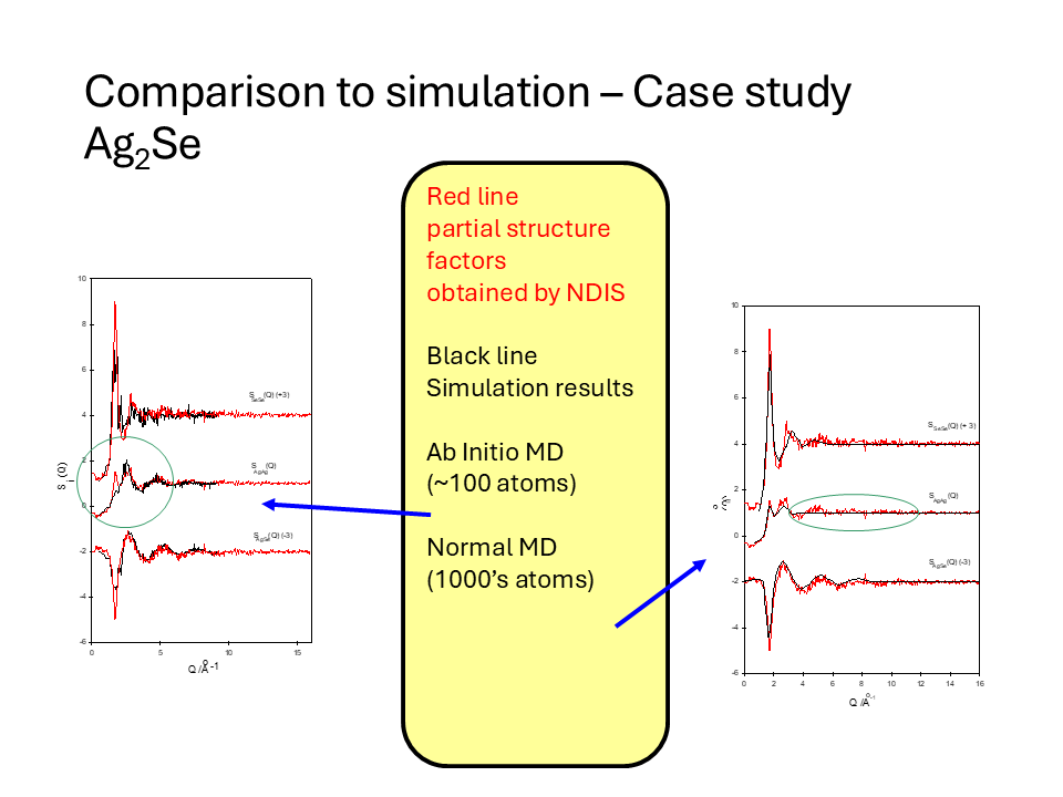
The ultimate aim of the experiment and simulations would be a structure that is self consistent with all the techniques exploited. Computer methods that are moving to this goal are the latest implementation of Reverse Monte Carlo fitting (where atomic positions in a model structure are continually adjusted to obtain good fits to, for example, diffraction and EXAFS data simultaneously) or the Empirical Potential Structural Refinement (EPSR) where molecular dynamic potentials are dynamically adjusted until the simulation agrees with experimental measurement.

20.11 Molecular materials

What happens when we wish to look at the structure of materials at a coarser scale than the atomic resolution, for example, large molecular or polymeric systems? This is an interesting question and might be phrased in a slightly different manner - at what point is it unnecessary to consider the atomic nature of a material? As you might imagine it is all a matter of scale. If I asked how the plastic balls in a child’s play pit arranged themselves it would be hard to expect you to give an interpretation based on interatomic potentials. I’d imagine them as rigid hollow spheres surrounded by a very low density fluid (air).

So, what techniques might we use as we move up from the scale of atoms (\(\sim\) 0.1 nm) to molecules (1-10 nm)? Well in our discussion of X-ray and neutron diffraction so far we saw that we needed to measure the scattering to quite wide angles (\(>90^\circ\)) in order to have enough range in \(Q\) to resolve the interatomic structure. If we look at the typical structure for a simple atomic liquid we see that the scattering at small \(Q\) becomes smaller and tends towards zero (not quite true - it depends on the compressibility) as \(Q\rightarrow 0\). Indeed, the first peak in our diffraction pattern is typically around \(Q\sim (2\pi/d)\) where \(d\) is the shortest interatomic distance. This reflects the observation that the peaks in \(g(r)\) steadily decrease as \(r\) increases. Now suppose we imagine our system consists of molecular spherical ‘balls’ of the order of 4 nm in diameter. Our wide angle diffraction pattern will arise primarily from all interatomic distances in the molecule. However, there will be large regions (the gaps between the balls) where there are no atoms to scatter the X-rays or neutrons. We have seen a similar situation before - X-rays are scattered from the electrons and the scattering from the atom was interpreted in terms of the X-ray form factor that describes the distribution of the electrons in the atom. For both neutrons and X-rays we now have an analogous situation, the scattering from our molecular ball will depend on the distribution of the scattering centres in our molecule that we can describe as a form factor for the molecule (like \(f(Q)\) for x-rays). If we imagine our diffraction pattern from our system of molecular balls we can see a diffraction peak corresponding to the inter ball (intramolecular) spacing at \(Q\sim 2\pi/4 \sim 1.5\) nm\(^{-1}\) (as the balls are 2 nm in radius and hence separated by 4 nm if they are in contact) superimposed on the decreasing molecular form factor followed by the interatomic part at high \(Q\).

So the answer to our question is that if we are studying molecular systems, for example, liquid crystals, micelles etc. then we need to either change our probe to use lower energy (longer wavelength) neutrons or X-rays or concentrate our efforts at measuring the diffraction pattern at small angles (or both). Hence, in principle, we could apply many of the transform techniques described above (but on a different length scale) \(\textit{provided}\) we know the molecular form factor. Unfortunately, molecules don’t generally form a nice ‘ball’, they are not necessarily spherical and they may distort so this won’t work! Sometimes useful approximations can be made - for example a typical idea is the radius of gyration (\(R_g\)) of the molecule i.e. approximating its scattering to a spherical object. However, the field of small angle scattering from molecular systems is vast and many approaches are taken to the analysis of results that we do not have time to cover.

Neutron scattering is also a very powerful technique for studying these systems. There is a very large difference in the scattering lengths of normal hydrogen \(^1_1H\) and its heavier deuterium isotope \(^2_1H\). By selectively ‘deuterating’ molecules or parts of molecules the scattering at small angles from two otherwise identical samples may be enhanced to highlight the structure of disordered molecular systems at this intermolecular mesoscopic scale - a technique that has been used extensively to understand and optimise materials for the food and cosmetic industries to name a few.

As we increase the size of our components the principles of diffraction stay the same - we aim to use wavelengths that are comparable to the size of the scattering objects. This is not always easy as other effects including absorption and refraction may come into play. However, it is possible to diffract radio waves from arrays of macroscopic reflectors for example and you are already very familiar with optical diffraction from 2D arrangements of diffracting objects with sizes comparable to the wavelength of light.

20.12 Summary and keypoints

As we approach atomic sizes attempts to measure structural properties in real space (\(g(r)\)) become harder and harder. In this regime the main tools for measuring structure are X-ray and neutron diffraction and perhaps electron diffraction in certain cases. In addition, spectroscopic measurements may be used and are sensitive to the local environments around different atom types.

In diffraction experiments important factors to consider are,

• the wavelength of the x-ray or neutrons,
• the maximum and minimum accessible \(Q\) value compared to the length scales being probed,
• the accessibility of the source (central facilities needed?),
• cost and availability of isotopes.

In spectroscopic experiments important factors include,

• the sensitivity of the technique for the atom type in question,
• cost and accessibility of the desired spectrometers,
• difficulty of analysing the data and the accuracy (rather than sensitivity) of the method for obtaining i.e. \(g(r)\).